Burst statistics in non-linear stochastic models

Time series obtained by solving non-linear stochastic models exhibit rather interesting statistical properties. On Physics of Risk we have already discussed some of these models [1, 2] (ex. stochastic model of return, herding model of financial markets), which are able to reproduce statistical properties of high frequency return (namely spectral density and probability distribution).

In statistical sense model and financial market behavior might be studied in many different manners. One may study probability distributions, moments, spectral densities, autocorrelations and etc., using each of them to obtain vital information on the statistical and dynamical properties of the studied system. It is important to note that new useful information might be provided by the statistical indicators, which are related to the previously used indicators in unambiguous manner. One may also introduce new variables describing system itself or its time series.

There is a group of such variables, which is closely related to the estimation of risk, known as burst statistics [3, 4]. In this text we will discuss these variables and their statistical properties. At the end of the text we also present an interactive HTML5 applet, using which one can reproduce burst statistics of certain stochastic model.

Burst statistics

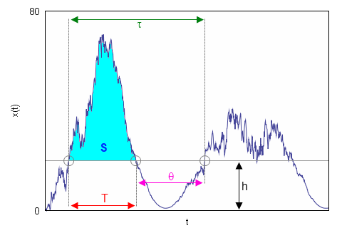
Before analyzing burst statistics we have first to define what these burst are. Evidently burst is a cluster of larger values in the time series, thus we must define some threshold value and assume that every point above it belong to burst. We denote threshold value as h (abbreviation of "height"). In Fig. 1 we have also marked three threshold passage events - start of the example burst, end of the example burst, start of the next to the example burst. These three events will be further referenced then introducing variables schematically introduced in Fig. 1.

Fig. 1:Variables related to the burst statistics: h - threshold value; τ - waiting time; T - burst duration; S - burst size; θ - inter-burst time.

As you can see in Fig. 1 we have denoted time window between first and third event as τ. We will call τ waiting time as it tells us the times between two successive bursts. Time interval between second and third event, θ, is similar variable, but it describes inter-burst times. Burst duration, time between first and second events, is denoted as T, while burst size, defined as area between threshold line and time series curve (cyan area in Fig. 1), is assigned symbol S (abbreviation of "size").

It is known that probability densities of τ, T and θ, obtained from non-linear stochastic models, can be fitted by power law. Furthermore it is known that characteristic burst size is proportional to the power of burst duration [3, 4]. Numerical evaluation of simple non-linear stochastic model,

\begin{equation} \mathrm{d} x = \left ( \eta - \frac{\lambda}{2} \right)\left( 1+x^2 \right)^{\eta-1} x \mathrm{d} t + \left( 1+x^2\right)^{\frac{\eta}{2}} \mathrm{d} W , \label{sde} \end{equation}

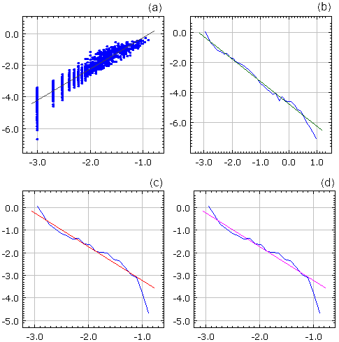
provides \( S \propto T^2 \), \( p(\tau) \sim\tau^{-1.5} \), \( p(T) \sim T^{-1.5} \), \( p(\theta) \sim \theta^{-1.5} \) relations, where p is probability density function of certain variable. It was shown that these relations hold for \( \eta \geq 1 \) case [4] and are very similar, power law nature is retained, but powers themselves slightly differ, in \( \eta <1 \) case [3]. Below, see Fig. 2, we have shown typical results obtained by using interactive applet provided at the end of this text.

Fig. 2:Burst statistics observed in non-linear stochastic model. All scales are lg-lg. (a) S versus T, (b) τ , (c) T and (d) θ probability densities. Blue dots are numerically obtained results, while differently colored lines fit them with power law. Slope, power, of gray line is 1.99, green line -1.54, red line -1.56 and magenta line -1.45. Program parameters: η=2.5, λ=3, Δt=0.001, h=2.

Eq. \eqref{sde} was derived while looking for stochastic model capable of reproducing empirical statistical properties of high frequency return [1] (see the corresponding text on Physics of Risk). Though this equation is simpler than final one, it is still able to reproduce power law distribution and long-range memory of return. Thus analysis of this equation in terms of burst statistics might provide useful insights for risk management.

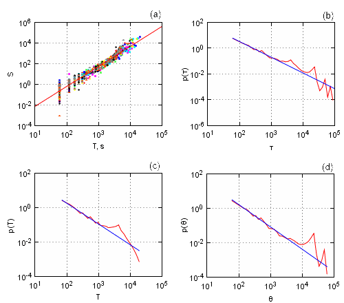
This presumptuous conclusion might be backed by empirical analysis. As solutions of Eq. \eqref{sde} have spectral density similar to the empirical spectral density, it is to be expected that empirical data should also have similar burst statistics. Indeed as you can see in Fig. 3 empirical data, we have analyzed 26 different stocks traded on New York Stock Change from January 2005 to March 2007, has similar burst statistics:

• In sub-figure (a) we have presented burst size versus burst duration plot. Different symbols correspond to different stocks (we have used 9 randomly selected stocks). As you can see symbols of all stocks lie in same region with little or no difference in positioning visible. Empirical data in this figure was fitted as power law, \( S \propto T^{1.94} \).
• In sub-figure (b) we have plotted average, averaged over 26 stocks, τ probability density function. Empirical data once again can be fitted by power law, \( p(\tau) \sim \tau^{-1.47} \).
• In sub-figure (c) we have plotted average, averaged over 26 stocks, T probability density function. Empirical data once again can be fitted by power law, \( p(T) \sim T^{-1.46} \).
• In sub-figure (d) we have plotted average, averaged over 26 stocks, θ probability density function. Empirical data once again can be fitted by power law, \( p(\theta) \sim \theta^{-1.52} \).

Fig. 3:Empirical burst statistics (h=1) of one minute absolute return time series, filtered by one hour moving average filter, of 26 varying stocks from New York Stock Exchange, traded from January 2005 to March 2007. (a) burst size versus burst duration of 9 randomly selected stocks, while (b), (c) and (d) are probability density plots. Empirical data was fitted by power laws with powers: (a) 1.94, (b) -1.47, (c) -1.46 ir (d) -1.52.

We have obtained results presented in Fig. 3 by analyzing one minute absolute return time series. All analyzed time series were filtered using one hour moving average filter prior to analysis. We have set burst threshold value to 1, h=1.

HTML5 applet

References

• V. Gontis, J. Ruseckas, A. Kononovicius. A Non-linear Stochastic Model of Return in Financial Markets. In: Stochastic Control, ed. C. Myers. InTech, 2010. doi: 10.5772/9748.
• A. Kononovicius, V. Gontis. Agent based reasoning for the non-linear stochastic models of long-range memory. Physica A 391: 1309-1314 (2012). doi: 10.1016/j.physa.2011.08.061. arXiv: 1106.2685 [q-fin.ST].
• M. Alaburda, B. Kaulakys. Simulation of bursting, rare and extreme events by nonlinear stochastic differential equations. Dynamics of Socio-Economic Systems 2: 175-182 (2011).
• B. Kaulakys, M. Alaburda, V. Gontis. Modeling scaled processes and clustering of events by the nonlinear stochastic differential equations. AIP Conference Proceedings 1129: 13-16 (2009).