Multifractality of time series

One of the conclusions of fractal geometry is a fact that fractals unlike traditional Euclidean shapes lack characteristic scale. Those "fractured" objects are self-similar - defining geometry is clearly visible on multitude of scales. It is known that self-similarity is observed not only in formally defined geometric objects, such as Sierpinski triangle or Koch snowflake, but also in the surrounding nature. One of my most favorite examples is a comparison of tree, its branches and a leaf (for more inspiring examples see introduction of Fractals section) - they all have branching structure and something green filling the extra space in between.

The interesting thing, in context of the topic in focus, is that one can extend fractal formalism beyond formal or natural geometric shapes. It is also noticed that some of the natural processes exhibit fractal features in their time series! It is known that geoelectrical processes [1], heartbeat [2] and even human gait [3] time series posses this feature. While financial market, frequently analyzed on Physics of Risk website, time series are also no exception [4, 5]. Though the aforementioned time series are much more complex - they exhibit not monofractality (single manner self-similar behavior as the aforementioned formal geometric fractals do), but multifractality!

Fractality of time series

In Physics, but not only in Physics, scale invariance is mostly associated with power law dependencies. One can put this idea down mathematically as:

\begin{equation} W(a t) = a^H W(t) , \end{equation}

where \( W(t) \) is some time series, \( a \) some scale shift, \( H \) characteristic scaling exponent. Equality of the left hand side and right hand side of equation doesn't need to be strict - in case of stochastic processes it might represent purely statistical similarity [6].

One of the most well known statistically self-similar processes is Brownian motion, which also known as Wiener process. It is known that Wiener process obeys Gaussian distribution with time dependent standard deviation, which increases overtime as square root of elapsed time - \( \sigma \sim \sqrt{t-t_0} = \sqrt{\Delta t} \). Thus we above relation holds for variance of Wiener process with \( H=0.5 \). It is worthy note that there is extension of this process known as fractional Brownian motion, which may be represented by different values of characteristic scaling exponent [6].

The problem of monofractality in the time series still remain as Wiener process, or its generalizations, is still described by single scaling exponent. While multifractal time series would be described by a set of scaling exponents [6, 7]. Nevertheless our understanding of fractality of time series should have improved as now we should be able to understand fractals, whose dimensions are not limited to spatial ones. Using this example we have also understood what statistical self-similarity stands for - it doesn't stand for strictly repeating shapes (as for example in aforementioned Sierpinsky triangle case), it stands for repetition of statistical properties, which describe observed random shapes.

As we have mentioned before we will be interested in processes with broad \( H \) spectrum. One can obtain it using varying methods [6, 8], while we will limit ourselves to presentation of only one, yet very common and popular, method - MF-DFA method [7].

Multifractal detrended fluctuation analysis (MF-DFA)

To begin with (step 1) the analysis of time series using MF-DFA method one should obtain the profile of time series:

\begin{equation} y_i = \sum_{k=1}^{i} [x_k - \langle x \rangle] , \quad i=1, 2, \ldots, N , \end{equation}

here \( y \) is profile, \( x \) is the analyzed time series, \( \langle x \rangle \) is its mean value, while \( N \) stands for the length of the series. Subtraction of mean is not necessary, yet it might facilitate (depends on the method used for detrending) calculations in further steps.

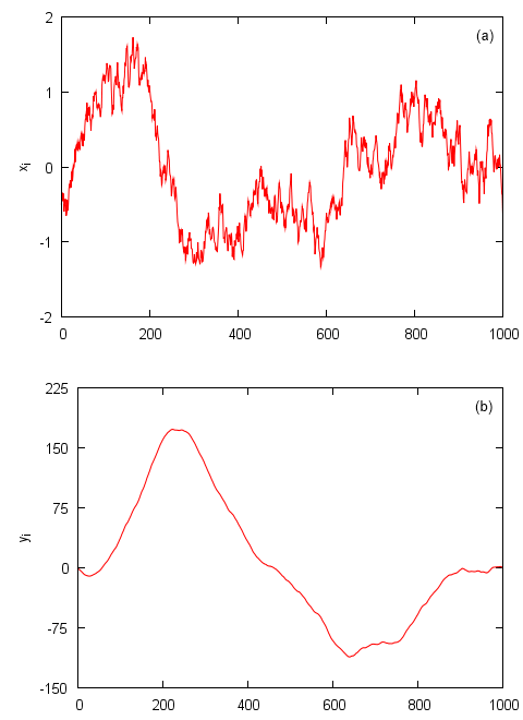Fig. 1:Step 1: stochastic time series (a) and its profile (b). Stochastic time series generated using standard Wiener process.

Afterwards (step 2) one should split profile series into separate non-overlaping segments with size \( s \). After this operation one should have \( N_s = \mathrm{int}(N/s) \) segments. For the most \( s \) there will be some leftover points, whose number is to small to form another segment. If we are not willing to lose information contained in them we should repeat the same process, namely splitting, from the end of the profile series. In such case we effectively double the number of segments - one should now have \( 2 N_s \) segments.

During the third step trends in all segments are estimated. Trends should be approximated by polynomial of the selected order. As there is no restriction for possible selection, one can choose any positive integer. MF-DFA title is appended based on the selected order. Thus if one uses parabolic (or square) fits, then one can say that MF-DFA2 is used. As it is problematic, in terms of computer resource and evaluation time, to fit data with higher order polynomials, in practice polynomials of first to third order are considered. For the sake of simplicity and ease of presentation we use MF-DFA1 method, namely we use linear least-square fits to detect and remove trends in the profile series.

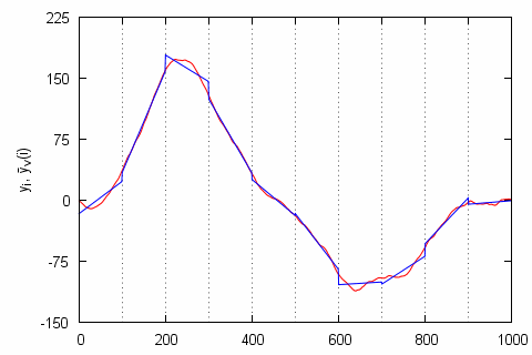Fig. 2:Steps 2 and 3: we have split the profile (red curve) into s=100 sized segments (splits are marked with dashed line) and estimated their trends (blue curve). The profile has remained the same as in , while the profile fits in each given segment are linear.

When the trends are known (step 4) we can remove them by subtracting them from the profile series. Mathematically for the segments, which were formed the start of the series, \( \nu = 1, 2, \ldots,N_s \), this can be expressed as:

\begin{equation} F^2_{\nu}(s) = \frac{1}{s} \sum_{i=1}^{s} \left[y_{(\nu-1) s +i} - {\bar y}_{\nu}(i) \right]^2 , \end{equation}

while for the remaining segments, \( \nu = N_s +1, \ldots, 2N_s \), same thing can be done like this:

\begin{equation} F^2_{\nu}(s)= \frac{1}{s} \sum_{i=1}^{s} \left[y_{N-(\nu-N_s) s +i} - {\bar y}_{\nu}(i) \right]^2 . \end{equation}

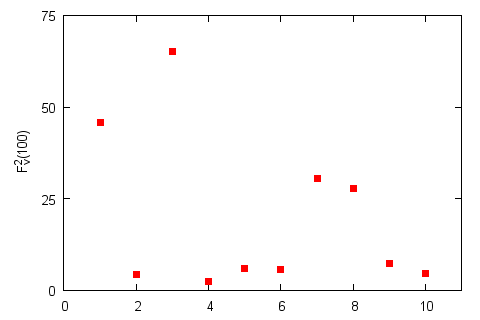Fig. 3:Step 4: \( F_ν^2(100) \) for the selected segments. Profile and its splits remain the same as in Fig. 2.

All what remains (step 5) is to average obtained fluctuations functions over all segments:

\begin{equation} F_q(s) = \left\{ \frac{1}{2 N_s} \sum_{\nu=1}^{2 N_s}\left[ F^2_{\nu}(s) \right]^{\frac{q}{2}}\right\}^{\frac{1}{q}}. \end{equation}

In the above \( q \) stands for generalized coefficient, which is the one enabling us to recover multifractal features - it is also the only difference from the original detrended fluctuation analysis (DFA) method [7]. It is worthy to note that \( q \) is a real number and if its value approaches zero the above relation diverges. Thus in such case one must substitute ordinary averaging procedure with exponential averaging:

\begin{equation} F_0(s) = \exp\left\{ \frac{1}{4 N_s} \sum_{\nu=1}^{2N_s} \ln\left[ F^2_{\nu}(s) \right] \right\}. \end{equation}

Finally (step 6) by changing \( q \) and \( s \), while once again iterating through steps 2, 3, 4 and 5, one obtains \( F_q(s) \) curves. From their plots on log-log scale one should be able to recover power law relations - \( F_q(s) \sim s^{h(q)} \) (here \( h(q) \) is a generalized exponent, which is related to the generalized Hurst exponents as \( H(q) = h(q) -1 \) (for non-stationary \( h(q)>1 \) time series) or \( H(q) = h(q) \) (for stationary series, \( h(q)<1 \))). If generalized exponents are constant or almost constant, then time series can be considered monofractal. While if \( h(q) \) dependence (or in other words spectrum) is rich, then time series can be considered multifractal.

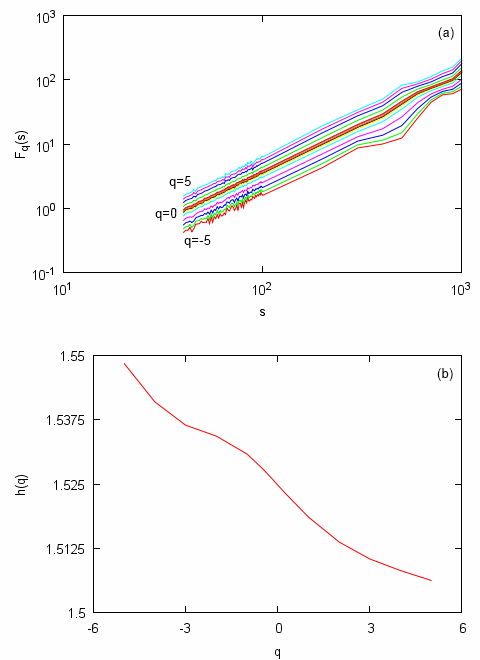Fig. 4:Steps 5 and 6: deviations from trends estimated for different segment sizes (a) and generalized exponent spectrum (b). Relations obtained from time series based on one presented in (original series extended to 32768 points).

In the above figures we have illustrated different MF-DFA steps by analyzing standard Wiener process. Thus the final result, Fig. 4, namely the observed monofractality of time series was not unexpected. Though at first glance it might occur that signal is multifractal as width of \( h(q) \) spectrum is non-zero as it should be according to the theory. This discrepancy is caused by the finite size of analyzed time series. Actually we have attempted to obtain \( h(q) \) spectrum in case of original, 1000 point wide, time series, but the obtained \( h(q) \) spectrum was unexpectedly broad - 0.2 (approximately 15% of the mean \( h(q) \)). While the multifractal analysis of the same yet extended, 32768 points wide, series (as you can see in Fig. 4) revealed narrower spectrum - 0.04 (approximately 2.5% of the mean). Literature [6, 7] suggests that in the infinite limit spectrum would converge to single dot.

Furthermore as we see in Fig. 5 \( h(q) \) spectrum of multifractal time series is far more broader - 1.1 (approximately 90% of the mean). Curves presented in Fig. 5 were obtained by analyzing time series generated by the Agent-based herding model of financial markets. Multifractal properties of this model were already studied with two different methods - GHHCF [9] and the very same MF-DFA [10]. Also note the difference in scaling of \( F_q(s) \) (Fig. 5 (a) and Fig. 4 (a)).

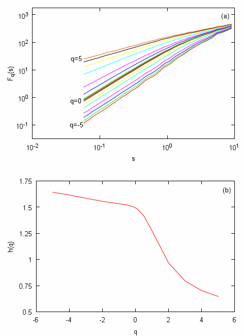Fig. 5:Multifractal features of Agent-based herding model of financial markets: deviations from trends estimated for different segment sizes (a) and generalized exponent spectrum (b). Model parameters: \( \varepsilon_1=\varepsilon_2=1 \), \( \Delta t=0.001 \), \( \tau(y)=1/y \).

Additional information visible in generalized exponent spectrum

Actually MF-DFA is a generalization of an older DFA method. In case of \( q=2 \) MF-DFA produces exactly the same results as ordinary DFA method would [7] - \( h(2) \) equals exponent \( h \) as it is understood in the original DFA framework. Therefore interpretations which have originated from DFA [11] might be also applied to the results obtained with MF-DFA.

Judging from \( h(2) \) time series might be [11]:

• anti-correlated, if \( h(2) < 0.5 \).
• uncorrelated (be related to white noise), if \( h(2) \simeq 0.5 \).
• positively correlated, if \( h(2) < 1 \).
• strongly positively correlated, if \( h(2) \simeq 1 \). Or in other words exhibit so-called pink, or \( 1/f \), noise. Such time series should exhibit other long range memory related properties. Note that we have obtained such results with time series from Agent-based herding model of financial markets (see Fig. 5).
• non-stationary or similar to random walk, if \( h(2) < 1.5 \).
• related to Brown noise or Wiener process, if \( h(2) \simeq 1.5 \). See Fig. 4.

The above discussion can might be briefly mathematically expressed as [11]:

\begin{equation} \gamma = 2 - 2 h(2) , \quad \beta = 2 h(2) - 1 , \end{equation}

here \( \gamma \) is negative correlation function exponent, while \( \beta \) is negative power spectral density exponent. Note that the above relations are strict in no way - they might hold for some short regions of dependence, of for example frequencies (in case of power spectral density).

It is important to note that actual \( h(q) \) might be negative, while MF-DFA is able to detect only its positive values. Though one can extend the detectable range of \( h(q) \) of repeating step 1 few times. After each repetition detected generalized exponents increases by 1, \( \tilde{h}(q) = h(q) + n \) (here \( \tilde{h}(q) \) is detected generalized exponent, \( h(q) \) actual generalized exponent and \( n \) is a number of step 1 repetition times), allowing one to analyze strongly anti-correlated time series. This property of generalized exponent also suggests what might be observed for \( h(2) > 1.5 \).

This discussion also leads to another interesting conclusion - if step 1 is skipped results obtained from MF-DFA method should also coincide with results obtained from GHHCF method. For example Brownian-like time series would have \( h(2) \) equal to 0.5. Though in such case it would a problem to differentiate between Pink and White noises. The corresponding time series would be almost indistinguishable - both very different dynamics would produce the same value of \( h(2) \), namely zero. Thus obtaining time series profile is very important step needed to be able to distinguish Pink and White noises.

Singularity, Hölder exponent, spectrum

Singularity spectrum is an alternative way to characterize multifractal series. It was derived to accompany standard textbook box counting formalism [8]. Box counting formalism is a relatively simple and for a long time very popular method to determine fractal features of analyzed objects (including spatial ones). Thus singularity spectrum has become a default way to characterize multifractal series.

Singularity spectrum, \( f(\alpha) \), can be obtained by transforming generalized scaling function defined in terms of box counting formalism, \( \tau(q) \). Note that \( h(q) \) may also be referred to as a scaling function (or scaling exponent), but it is defined in the terms of MF-DFA or DFA, not in the terms of box counting formalism. Though it is known that both scaling exponents are related [7]:

\begin{equation} \tau(q) = q h(q) -1 . \end{equation}

By transforming, using Legendre transform, \( \tau(q) \) one obtains [7]:

\begin{equation} \alpha = \partial_q \tau(q) = h(q) + q \partial_q h(q) ,\quad f(\alpha) = q \alpha - \tau(q) = q \left[ \alpha - h(q)\right] +1 , \end{equation}

here \( \alpha \) is Hölder exponent, which describes the strength of singularity, while \( f(\alpha) \) denotes the dimension of the subset of the series described by certain Hölder exponent [7]. In Fig. 6 we clearly see large difference between the detected multifractality of the analyzed models/processes - singularity spectrum of Agent-based herding model of financial markets time series has broad spectrum of Hölder exponents, while Wiener process has very thin spectrum.

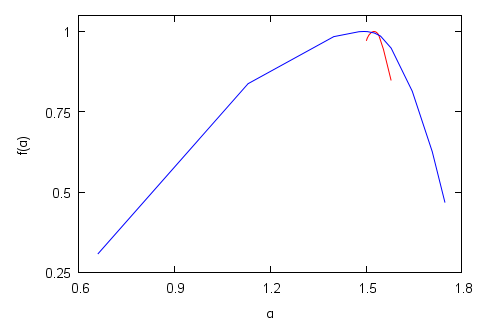Fig. 6:Singularity spectrum: standard Wiener process (red curve) and Agent-based herding model of financial markets (blue curve). Parameters of Agent-based herding model of financial markets were set as follows: \( \varepsilon_1=\varepsilon_2=1 \), \( \Delta t=0.001 \), \( \tau(y)=1/y \).

In scientific literature singularity spectrum is also frequently called Hölder exponent spectrum [6].

Applet

GUI of the applet below is reminiscent of the previous applet, which was published together with the text on Agent-based herding model of financial markets. Thus there is no point in discussing its input parameters. Furthermore most of the input parameters are directly related to the model discussed in the same text.

The only important differences are that this applet outputs multifractality spectra and that it allows to deform model time series. It is possible to remove correlations by shuffling time series and distort the underlying distribution (values are remapped to the \( [0,1] \) value region). Deformation of time series is very important and useful function as multifractal features might be observed due to correlations (model dynamics) and broad underlying distribution [7]. It is also known that multifractality can be influenced by the number of agents in the agent-based model [12], though we don't analyze this as it is already firmly confirmed that in this model dependence of multifractality on the number of agents is negligible [10].

References

• L. Telesca, V. Lapenna, M. Macchiato. Multifractal fluctuations in earthquake-related geoelectrical signals. New Journal of Physics 7: 214 (2005). https://iopscience.iop.org/1367-2630/7/1/214/fulltext.
• P. Ch. Ivanov, L. A. N. Amaral, A. L. Goldberger, S. Havlin, M. B. Rosenblum, Z. Struzik, H. E. Stanley. Multifractality in healthy heartbeat dynamics. Nature 399: 461-465 (1999).
• B. J. West, N. Scafetta. Nonlinear dynamical model of human gait. Physical Review E 67: 051917 (2003).
• E. E. Peters. Fractal market analysis: applying chaos theory to investment and economics. John Wiley and Sons, 1994.
• J. Kwapien, P. Oswiecimka, S. Drozdz. Components of multifractality in high-frequency stock returns. Physica A 350: 466-474 (2005). arXiv: cond-mat/0411112 [cond-mat.other].
• R. H. Riedi. Multifractal Processes. In: Long range dependence: theory and applications, ed. P. Doukhan, G. Oppenheim, M. S. Taqqu, pp. 625-715. Birkhauser, Boston, 2002. https://www.stat.rice.edu/~riedi/Publ/PDF/MP.pdf.
• J. W. Kantelhardt, S. A. Zschiegner, E. Koscielny-Bunde, S. Havlin, A. Bunde, H. E. Stanley. Multifractal detrended fluctuation analysis of nonstationary time series. Physica A 316: 87-114 (2002). arXiv: physics/0202070 [physics.data-an].
• J. Feder. Fractals. Plenum Press, New York, 1988.
• A. Kononovicius, V. Gontis. Agent based reasoning for the non-linear stochastic models of long-range memory. Physica A 391: 1309-1314 (2012). doi: 10.1016/j.physa.2011.08.061. arXiv: 1106.2685 [q-fin.ST].
• A. Kononovicius, V. Gontis. Mikroskopinis stochastinių modelių aiškinimas. 39-oji Lietuvos nacionalinė fizikos konferencija: Programa ir pranešimų tezės, p. 34. Vilnius, Lietuva, 2011.
• S. V. Buldyrev, A. L. Goldberger, S. Havlin, R. N. Mantegna, M. E. Matsa, C. K. Peng, M. Simons, H. E. Stanley. Long-range correlation properties of coding and noncoding DNA sequences: GenBank analysis. Physical Review E 51: 5084-5091 (1995). https://link.aps.org/doi/10.1103/PhysRevE.51.5084.
• F. S. Passos, C. M. Nascimento, I. Gleria, S. da Silva, G. M. Viswanathan. Fat tails, long-range correlations and multifractality as emergent properties in nonstationary time series. EPL 93: 58006 (2011). doi: 10.1209/0295-5075/93/58006.