Numerical methods for the stochastic differential equations

Reviewers of one of our most recent papers have asked some very interesting questions. One of them was about the numerical methods we use to solve the stochastic differential equations. The question was to be expected as, while we provide the final difference equations, we do not discuss how they were obtained. Thus here we will briefly review the most basic principles of the numerical solution of the stochastic differential equations.

Let us recall that in general case stochastic differential equation looks like:

\begin{equation} \mathrm{d} x = f(x) \mathrm{d} t + g(x) \mathrm{d} W. \end{equation}

The above can be even more general if the drift and diffusion functions would also depend on time, but in the most applied stochastic models there is no direct dependence time.

Euler method for the differential equations

Before tackling stochastic differential equation let us recall how one can numerically solve first order ordinary differential equations. The most intuitive and simple method is known as Euler method or first order numerical discretization method. In our case, while neglecting diffusion term, we obtain:

\begin{equation} \Delta x = f(x) \Delta t \quad \Rightarrow \quad x_{i+1} =x_i + f(x_i) \Delta t . \end{equation}

To understand what have we done here recall the definition of derivative:

\begin{equation} \frac{\mathrm{d} x(t)}{\mathrm{d} t} = \lim_{\Delta t\rightarrow 0} \frac{x(t) - x(t-\Delta t)}{\Delta t} \approx\frac{\Delta x}{\Delta t} . \end{equation}

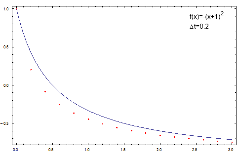
It should be evident that if the diffusion function is constant, namely if the correct answer linear, then Euler method is precise. While if the diffusion function does vary, namely if the correct answer is non-linear, then the differences between the numerical solution and correct answer will be noticeable. The deviation will depend on the size of the time step - if it is small, the deviation will also tend to be smaller.

Fig 1.Illustration of the Euler method applied towards non-linear differential equation. Note that the numerical solution (red dots) doesn't fully coincide with the correct answer (blue curve).

In Fig. 1 the differences between the numerical and correct answer are easily noticeable. In order to improve numerical results one can decrease the time step (which was selected to be large on purpose) or use another, more precise, numerical method. One of the possible choices, in order to retain speed of the numerical evaluation, would be midpoint method, which is an improved version of the first order Euler method considered in this text. In order to further improve the precision one should become interested in higher order methods - ex. Runge-Kutta 4-th order method. Another interesting idea might be implementation of variable time steps (see further).

Euler method for the stochastic differential equations

Let us now apply the ideas above towards stochastic differential equations! First let us substitute the differentiation with the changes of variables during some time window. By doing so we obtain the following difference equation:

\begin{equation} x_{i+1} = x_i + f(x_i) \Delta t + g(x_i) \Delta W . \end{equation}

The difference equation has a very familiar shape and the only unanswered question is about W process. Here W is a standard Brownian motion - path (coordinate) of the one dimensional particle influenced by some random force. As the total influence of many random factors follows the normal distribution, it is to be expected that the change of particles coordinate will follow normal distribution. The standard deviation will depend on time window width, actually the standard deviation will increase as a root of time window width. In such case we can rewrite the difference equation as follows:

\begin{equation} x_{i+1} = x_i + f(x_i) \Delta t + g(x_i) \sqrt{\Delta t}\zeta_i . \end{equation}

Here we purely intuitively arrive at numerical method which is known as Euler-Maruyama method. For more details on this method and its alternatives see reference [1].

Solving non-linear stochastic differential equations using variable time step

Note that Euler-Maruyama method works fine if the stochastic differential equation is at most linear or the diffusion area of the variable is somehow restricted. In case of the non-linear equations one can decrease the time step used to numerically solve the equation. Though note that this will significantly increase the required computer resources. Such choice would not be very optimal as the small time step is actually needed only if the movement, either drift or diffusion, of the random variable is large. It would be very intuitive and rational to use variable time steps! This way it would be possible to decrease computational load if it is not necessary.

Let us now consider the following non-linear stochastic differential equation:

\begin{equation} \mathrm{d} x = \left(\eta - \frac{\lambda}{2} \right)x^{2 \eta -1} \mathrm{d} t + x^\eta \mathrm{d} W . \end{equation}

We choose this equation as it represents very general class of stochastic differential equations [2, 3] and it lies in the base of the stochastic models derived and studied by our group [4, 5]. Furthermore in some distinct cases this equation becomes very similar to some very well known stochastic processes (we will discuss this in the following texts).

Following the previous ideas we can rewrite our non-linear stochastic differential equation as the following difference equation:

\begin{equation} x_{i+1} = x_i + \left(\eta - \frac{\lambda}{2} \right)x_i^{2 \eta -1} \Delta t + x_i^\eta \sqrt{\Delta t} \zeta_i . \end{equation}

Note the powers of random variable in the drift and diffusion terms. Also take note of the powers of time step. By comparing them we can that if the time step would be a function of random variable we could linearize the difference equation. Though now we will have to deal with two difference equations (one for the random variable, another for the time):

\begin{equation} x_{i+1} = x_i + \kappa^2 \left(\eta - \frac{\lambda}{2}\right) x_i + \kappa x_i \zeta_i , \end{equation}

\begin{equation} t_{i+1} = t_i + \kappa^2 x_i^{2- 2 \eta} . \end{equation}

Note that now the equations includes \( \kappa \), which stands for the numerical precision. Ideally it should be as small as possible, but in most of the cases 0.1 or 0.01 are ok.

This difference equation can be already solved numerically. Yet some problems might occur - e.g., for \( \eta>1 \) and small values of random variable the time step might become very large. This problem might be solved by switching back to the constant time step (of course only if its smaller than the variable one). Another frequent problem is related to the overly large or small values, which potentially can cause freezes, overflows or underflows, but this is another more technical topic.

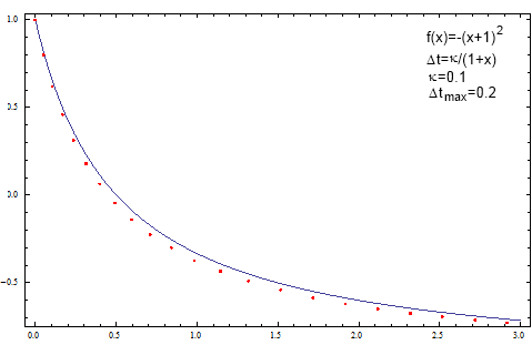
The idea of the variable time steps can be easily and somewhat efficiently applied towards solution of the ordinary differential equations - see Fig. 2.

Fig 2.Introducing variable time steps into the original Euler method. Note that under similar conditions the agreement between analytical and numerical solution is improved.

Source code as an example

Take time to familiarize yourself with the example Java program.

    public double step(double dt) {
        double t=0;
        while(t<dt) {
            double innerDt=variableTimeStep(lastX);
            if(Double.isNaN(innerDt) || Double.isInfinite(innerDt)) {
                innerDt=dt+dt-t-t;
            }
            double whileDt=Math.min(dt-t,innerDt);
            lastX=solveSDE(lastX,whileDt);
            t+=whileDt;
        }
        return lastX;
    }
    private double drift(double x) {
        return (eta-lambda/2.0)*Math.pow(x,2.0*eta-1.0);
    }
    private double diffusion(double x) {
        return Math.pow(x,eta);
    }
    private double solveSDE(double x, double dt) {
        return x+drift(x)*dt+diffusion(x)*Math.sqrt(dt)
            *gen.nextGaussian();
    }
    private double variableTimeStep(double x) {
        return Math.pow(kappa,2.0)*Math.pow(x,2.0-2.0*eta);
    }

References

• P. E. Kloeden, E. Platen. Numerical Solution of Stochastic Differential Equations. Springer, Berlin, 1999.
• J. Ruseckas, B. Kaulakys. 1/f noise from nonlinear stochastic differential equations. Physical Review E 81: 031105 (2010). arXiv: 1002.4316 [nlin.AO].
• J. Ruseckas, B. Kaulakys. Tsallis distributions and 1/f noise from nonlinear stochastic differential equations. Physical Review E 84: 051125 (2011). arXiv: 1111.2995 [cond-mat.stat-mech].
• V. Gontis, J. Ruseckas, A. Kononovicius. A Non-linear Stochastic Model of Return in Financial Markets. In: Stochastic Control, ed. C. Myers. InTech, 2010. doi: 10.5772/9748.
• A. Kononovicius, V. Gontis. Agent based reasoning for the non-linear stochastic models of long-range memory. Physica A 391: 1309-1314 (2012). doi: 10.1016/j.physa.2011.08.061. arXiv: 1106.2685 [q-fin.ST].