Describing high-frequency trader's behavior in the order book

We continue our series of posts on order book models by considering an order book model proposed by a group of scientists from Japan [1, 2, 3], which is based on high resolution data from foreign exchange market. Their work is extremely interesting as it starts from the empirical observations at the lowest level observable and is built up to reproduce some empirical observations at the higher levels. Also the model is analytically tractable using kinetic theory.

Brief description of the HFT model

The paper which describes the HFT model in detail [2] is rather long and involves a lot of sophisticated details explaining why the model was built as it was. Hence for the sake of brevity we will skip most of the discussion and mention only essential ideas.

The paper draws analogy between the kinetic theory in Physics and order book dynamics in Finance. Physical system can be "solved" by going between the three "hierarchical" description levels: micro-level particle motion (described by the Liouville equation), meso-level dynamics (described by the Boltzmann equation) and macro-level tracer particle motion (Brownian motion). The authors claim to obtain the same hierarchies for the financial markets and show the mathematical correspondence between the problems. Graphically they explain this idea by the figure we present to you a bit lower (the figure is a screenshot of the Fig. 1 from the [2]). This idea provides a background for the experimental (data analysis) setup as well as analytical treatment of the model.

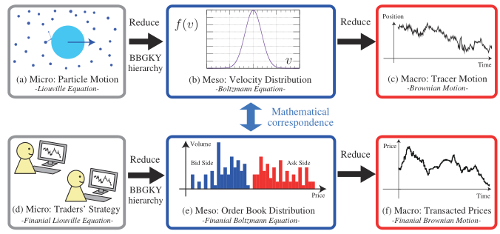Fig 1.The main idea of the model as illustrated by Kanazawa et al.

After performing the empirical analysis of high resolution order-book level data, the researchers determined four key features of the HFTs (abbr. high-frequency traders):

1. HFTs submit small number of live orders and the volume of the orders is small. Unlike low-frequency traders HFTs usually submit unit volume limit orders.
2. HFTs are liquidity providers. They are required to keep quotes in both bid and ask sides of the order book.
3. HFTs frequently modify their quotes. The researchers report that typical transaction interval was 9.3 seconds in their data set, while the quotes were typically modified within a second intervals.
4. HFTs follow recent price trends. On average HFTs modify their quotes by:

\[ \langle \Delta q \rangle \approx c_i \tanh \frac{\Delta p}{\Delta p_i^{*}} . \]

Having in mind these four observations the researchers consider a fixed number \( N \) of agents (representing HFTs) who submit both bid and ask limit orders. As agents submit to the both sides of the order book they can be characterized by their bid and ask quotes (\( b_i \) and \( a_i \) respectively) or by their own mid-price and spread (\( z_i = ( b_i + a_i ) /2 \) and \( L_i = b_i - a_i \) respectively). The second choice is more convenient as then we have only one temporal random variable \( z_i \), while \( L_i \) can be treated as an agents intrinsic property (also sampled randomly for each different agent, but constant in respect to time).

Empirical analysis shows that \( L_i \) is distributed according the Gamma distribution with shape parameter \( \alpha+1 \) equal to \( 4 \) and scale parameter \( L^{*} \) equal to \( 15.5 \). Without inputting these numbers the PDF of agent spread, \( L_i \), has the following form:

\[ p( L ) = \frac{L^{\alpha}}{ \Gamma(\alpha+1) L^{*(\alpha+1)}} \exp\left( - \frac{L}{L^{*}} \right). \]

Requotation due to recent prices trends (fourth observation) is included into the model as stochastic differential equation describing the motion of each agent's mid-price \( z_i \):

\[ \mathrm{d} z_i = c \tanh \frac{\Delta p}{\Delta p^{*}} \mathrm{d} t + \sigma \mathrm{d} W , \]

here the three parameters \( c \), \( \Delta p^{*} \) and \( \sigma \) ought to be different for each agent, but without loss of generality we can set them to identical typical values for all agents. Note that \( \Delta p \) changes discretely in time (each time transaction occurs its value is reset).

Finally we have to define "transaction rule" - how the quotes change after the transaction occurs. Lets assume that transaction has occurred, because the following match was found:

\[ b_j = a_i . \]

After the transaction a new price is set \( p = ( b_j + a_i) /2 \) and price trend indicator value is set to \( \Delta p = p^{new} - p^{old} \). After this the traders are assumed to requote their orders simultaneously by setting their mid-prices to the transaction price. This induces a momentary movement of agent's \( j \) quotes by \( - L_j/2 \) and agent's \( i \) quotes by \( L_i /2 \).

To visually understand how the model behaves see an illustration by Kanazawa et al. below (the figure is a screenshot of Fig. 4 from the [2]).

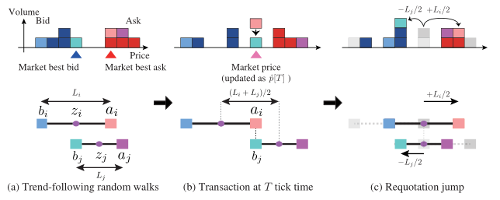Fig 2.Schematic representation of the model as illustrated by Kanazawa et al.

Weak, strong and marginal trend following regimes

This model exhibits three distinct behavioral regimes based on how much impact trend following has. The strength of trend following is well captured by the \( \tilde c \) parameter, which depends on the model parameters as follows [1, 2]:

\[ {\tilde c} =\frac{c L^{*} \sqrt{\alpha (\alpha-1)}}{\sigma^2 \sqrt{2 N}} . \]

As the model is based on empirical observations Kanazawa et al. [1, 2] estimated the parameter values from their data set. These values are the default ones in the figures (app screenshots) and app below: \( c = 6 \), \( \Delta p^{*} = 7.5 \) , \( \sigma=3.8 \) (authors do report a different value, but I believe that this is a mistype on their part as in that case \( \tilde c \) value would not be a correct one), \( \alpha=3 \) and \( L^{*}=15.5 \). We have used \( N = 100 \) in all our simulations, which consistent with the data set used in the original paper.

If \( \tilde c \) is significantly smaller than 1, then trend following is weak. In this case diffusive behavior of the HFTs dominates, hence the price change distribution is approximately Gaussian. Auto-correlation function for the short lags is noticeably negative.

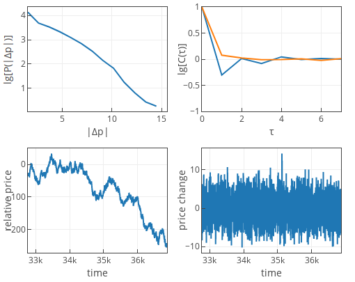Fig 3.Weak trend following (default parameters, except \( \sigma=14.5 \)).

If \( \tilde c \) would be significantly larger than 1, then trend following is strong. In this case drift behavior of the HFTs dominates. The price change PDF is exponential, while auto-correlation function for the short lags is noticeably positive. The auto-correlation function in our app below is positive, if last 1024 time ticks (points) include at least one trend reversal. If the current trend persists for longer than 1024 points, then auto-correlation function will fluctuate around zero. This is just minor artifact of the algorithm we implemented in the app.

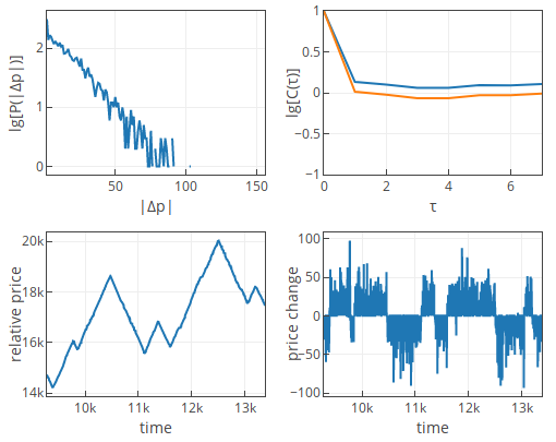Fig 4.Strong trend following (default parameters, except \( \sigma=1.8 \)).

If \( {\tilde c} \approx 1 \), then trend following is marginal. In this case we observe interplay between the drift and diffusion terms of the HFTs. The price change PDF is exponential. While the auto-correlation function will fluctuate around zero. For some parameter sets it will favor negative side, for some - positive side.

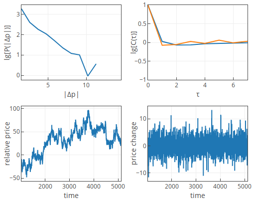Fig 5.Marginal trend following (default parameters).

The empirical estimates point to the third case. The paper reports that marginal following case is also consistent with empirical facts (price change PDF and auto-correlation for the short times).

Interactive applets

To understand the model and its dynamics better you should study the interactive applets below.

The first applet, as has become usual, shows us how the structure of the order book evolves as the time goes on. Note that unlike in most other cases here we have relative price on the x axis, thus negative "prices" will also be observed. Also note that this model uses continuous prices, hence the plot below shows a number of submitted limit orders in the interval \( [ p, p+1 ) \). Note that the shape of the both sides of the order book is symmetric and has shape similar to the log-normal distribution (similarly as in the previously discussed model), but the true expression is different [1, 2].

The second applet is in certain sense traditional Physics of Risk applet for all financial market models. Only now every plot was changed somewhat to show the important feature of this model.

First of all this model uses relative price instead of log-price or price and "price change" instead of returns. Relative price is measured as a distance in price ticks from some arbitrarily selected "zero" level. "Price change", \( \Delta p \) is measured as a difference between relative prices at two different points in time (the temporal distance, \( \Delta t \), between these points is kept constant for consistency).

This model exhibits statistical properties which are different from the ones we are usually interested in. In this model the price change is distributed either normally or exponentially (depending on the parameter values), hence the PDF plot features log-linear axes instead of log-log axis we usually use.

Also instead of plotting power spectral density we plot auto-correlation, \( C ( \tau ) \), function of the price change. \( C ( 0 ) \) will be always equal to 1, but other nearby values will behave different depending on the parameter values. For the sake of speed, we consider only 1024 last time series points when calculating auto-correlation function, so some "artifacts" may appear. Note that we show two curves, which will most of the time over lap. The blue curve shows auto-correlation of the price change time series, while the yellow curve shows auto-correlation of the absolute price change time series.

Acknowledgment. This post was written while reviewing literature relevant to the planned activities in postdoctoral fellowship ''Physical modeling of order-book and opinion dynamics'' (09.3.3-LMT-K-712-02-0026) project. The fellowship is funded by the European Social Fund under the No 09.3.3-LMT-K-712 ''Development of Competences of Scientists, other Researchers and Students through Practical Research Activities'' measure.

References

• K. Kanazawa, T. Sueshige, H. Takayasu, M. Takayasu. Derivation of the Boltzmann Equation for the Financial Brownian Motion. Physical Review Letters 120: 138301 (2018). doi: 10.1103/PhysRevLett.120.138301. arXiv: 1703.06739 [q-fin.TR].
• K. Kanazawa, T. Sueshige, H. Takayasu, M. Takayasu. Kinetic Theory for Finance Brownian Motion from Microscopic Dynamics. arXiv: 1802.05993 [q-fin.TR].
• A. G. Smart. The statistical mechanics of currency exchange. Physics Today, 2018-04-23. doi: 10.1063/PT.6.1.20180423a.