Non-stationary power-law in a kinetic "rich gets richer" model

More than four years ago I (Aleksejus) started a series of posts reviewing with most well known kinetic exchange models. Recently I had to refresh my memory on this topic as a colleague (Julius) suggested an idea how to obtain power-law from the constant exchange model.

Initial idea

The idea was to remove agents which have lost all of their wealth. Obviously this model converges to a fixed state, in which one agent has accumulated all wealth. Namely, the model would not have an interesting stationary distribution, but the colleague expected to obtain power-law just before the simulation reaches the fixed state. The idea did not work out - the model produces something similar to Gaussian distribution which gets narrower as the simulation reaches the fixed state.

I have implemented the model in Python. The code follows. You could run this model multiple times to average out the time-dependent distribution (to obtain a smoother solution).

import numpy as np

def evaluateModel(nAgents,initialWealth,nSteps):
    wealth=np.zeros(nAgents)+initialWealth
    for i in range(nSteps):
        try:
            iPair=np.random.choice(nAgents,size=2,replace=False)
            if(wealth[iPair[0]]>0 and wealth[iPair[1]]>0):
                wealth[iPair[0]]+=1
                wealth[iPair[1]]-=1
        except ValueError:
            return wealth
    return wealth

Alternatively one can write the following set of equations and solve them numerically: \begin{equation} P_{0,t+1}=P_{0,t}+\frac{1}{N}P_{1,t}, \end{equation} \begin{equation} P_{1,t+1}=P_{1,t}-\frac{2}{N}P_{1,t} + \frac{1}{N}P_{2,t}, \end{equation} \begin{equation} P_{i,t+1}=P_{i,t}-\frac{2}{N}P_{i,t} + \frac{1}{N}P_{i-1,t} + \frac{1}{N}P_{i+1,t}, \quad \forall i \in \mathbb{Z}: 1 < i < W-1 , \end{equation} \begin{equation} P_{W-1,t+1}=P_{W-1,t}-\frac{2}{N}P_{W-1,t}+\frac{1}{N}P_{W-2,t}, \end{equation} \begin{equation} P_{W,t+1}=P_{W,t}+\frac{1}{N}P_{W-1,t}, \end{equation} in the above \( P_{i,t} \) is a fraction of agents having wealth \( i \) at time \( t \), while \( W \) is a total wealth of all agents combined (\( W = N W_0 \)). The initial condition for these equations is: \begin{equation} P_{i,0} = \delta(W_0-i) . \end{equation} Solving these equations allows to obtain the same result, but noticeably faster. Python code solving these equations is given below. Note that this function returns a histogram and not an array of agents' wealth as the other functions in this article.

import numpy as np

def evaluateModel(nAgents,initialWealth,nSteps):
    totalWealth=nAgents*initialWealth
    wealth=np.zeros(totalWealth+1).astype(float)
    wealth[initialWealth+1]=1.0
    for j in range(nSteps):
        newWealth=np.zeros(len(wealth))
        for i in range(len(wealth)):
            if(i>0 and i<totalWealth):
                newWealth[i-1]+=wealth[i]/nAgents
                newWealth[i]+=(wealth[i]-2.0*wealth[i]/nAgents)
                newWealth[i+1]+=wealth[i]/nAgents
            elif(i==0 or i==totalWealth):
                newWealth[i]+=wealth[i]
        wealth=newWealth.copy()
    return wealth

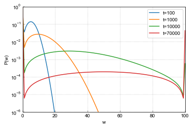
Note that this formulation not only helps to obtain the results faster, but also reveals that the initial model is equivalent to a Brownian motion with absorbing boundaries. This provides intuition on how the temporal solutions should look like. And what we get from numerical simulation matches the theoretical expectation (see figure below).

Fig. 1:Evolution of the distribution of wealth in the initial model. The PDF becomes broader and its middle peak value starts to move to the middle. After some time it starts to decline and boundary peaks (at 0 and total wealth) start to become more prominent. Figure was obtained by setting nAgents=25, wealth=4 and nSteps to the specified t values.

"Rich gets richer" modification

Let us modify the model by introducing rich gets richer dynamics, in a spirit of the Barabasi-Albert model, into our kinetic model. Namely, the probabilities for the agent to be picked are no longer equal, they are proportional to the agent's wealth. This small change does not influence the outcome of the model - it will still arrive to a fixed state, but it will arrive at a different manner.

Note that previously we always transferred wealth to the first agent we picked and subtracted wealth from the second agent. Although this seems to be unfair (or illogical), but as the selection probabilities were equal, it was equally possible to pick agent A and then agent B and vice versa. Now as the probabilities are wealth-dependent the probabilities of AB and BA are not equal if agents have different wealth. If A is richer, then AB will be more likely than BA. We keep this "unfairness" in the modified model.

The implementation of the modified model in Python follows.

import numpy as np

def evaluateModel(nAgents,initialWealth,nSteps):
    totalWealth=initialWealth*nAgents
    wealth=np.zeros(nAgents)+initialWealth
    for i in range(int(nSteps)):
        try:
            agents=np.random.choice(nAgents,size=2,replace=False,
                                    p=wealth/totalWealth)
            wealth[agents[0]]+=1
            wealth[agents[1]]-=1
        except ValueError:
            return wealth
    return wealth

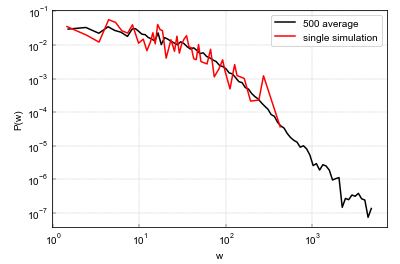
Fig. 2:The PDF of non-zero wealth for a model with nAgents=1000, initialWealth=5 and nSteps=235000. The PDF was averaged over 500 simulations.

This model produces what seems to be a power-law, but in order to clearly observe it one needs to run many simulations and average them out. So in the end it is not clear whether the model truly produces power-law or it is just a result of some undesirable effect (e.g., non-ergodicity). Note that if we drop the aforementioned "unfairness" model no longer produces power-law, so it is an important feature of the model. Also the specification of the model seems to be a bit unrealistic. Hence, we decided that while the model does not seem to merit a publication, it would seem to be an interesting topic to cover in Physics of Risk.