Poll-delayed voter model

In the yearly overview, I mentioned that I wanted to write a few posts about [1]. The model introduced in [1] is particularly interesting because it breaks the core assumption of the original voter model. In the "poll-delayed voter model" the agents do not interact directly with each other. Instead, they become aware of the opinion distribution in society through the periodic public polling.

Let us see what we can learn from this model.

Model

The noisy voter model is driven by independent exploration of the opinion space by the agents (switching event rate is given by \( \sigma_i \) where the index stands for the destination state) and by imitation of the peers (switching event rate is proportional to parameter \( h \)). Total birth (generation) and death (recombination) rates in respect to the number of agents in state "1", \( X\), are given by:

\begin{equation} \lambda\left(X\rightarrow X+1\right)=\lambda^{+}=\left(N-X\right)\left[\sigma_{1}+h X\right], \end{equation}

\begin{equation} \lambda\left(X\rightarrow X-1\right)=\lambda^{-}=X\left[\sigma_{0}+h\left(N-X\right)\right]. \end{equation}

It is trivial to see that the imitation process can be aligned with the reference clock. In other words, we can eliminate \( h \) by rescaling time, \( t \rightarrow h t \). The rescaled independent transition rates are then given by \( \varepsilon_i = \frac{\sigma_i}{h} \).

The total birth and death rates for the poll-delayed voter model take the following form:

\begin{equation} \lambda_{k}^{+}=\left(N-X\right)\left[\varepsilon_{1}+A_{k-1}\right], \end{equation}

\begin{equation} \lambda_{k}^{-}=X\left[\varepsilon_{0}+\left(N-A_{k-1}\right)\right]. \end{equation}

The most important difference from the noisy voter model is that the transition rates incorporate \(A_k\) instead of \(X\). This variable helps us denote incorporation of polling and delays. Let us define it as:

\begin{equation} A_k = X \left( k \tau \right). \end{equation}

In the above \( k \) would stand for the number of the poll, and \( \tau \) is the polling period (which is also aligned with announcement delays). In the real time, last revealed poll information is given by:

\begin{equation} A_{k-1} = A_{-1} \left( t \right) = X \left( \left\lfloor \frac{t}{\tau} - 1 \right\rfloor \tau \right). \end{equation}

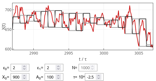
The figure below, and the app even further down, serve as an illustration to the logic behind the model. In both the red curve represents the evolution of the system state, \( X \). The other curves represent data gathered during the polls: the black curve show the most recently announced poll result, \( A_{k-1} \), while the gray curve indicates the most recent poll outcome, \( A_{k} \). It is important to stress that \( A_{k-1} \) is already public information, while \( A_{k} \) is still being processed by the pollster. At the beginning of each polling period, at \( t=k\tau \), the gray curve intersects both the red and black curves. This indicates that the results of the latest poll are being made public, and the new poll information is collected for processing. Between the polls, the red curve fluctuates, generally trending towards the black curve, reflecting how the system state incorporates the most recent public information.

Fig. 1:Sample trajectory of the poll-delayed voter model.

Numerical simulation of the model

In general, the noisy voter model can be simulated using the Gillespie method [2]. Still, in this case, one would need to modify it heavily [1]. Another concern is the speed of the Gillespie method. For the poll-delayed voter model, it is just too slow. Especially for the longer polling periods.

Hence, in [1], we have proposed an alternative model, which makes use of the convenient observation that \( A_{k-1} \) remains constant in between the polls. Thus, there is little difference between the independent exploration and peer imitation between the polls. We can encompass both mechanisms within effective independent transition rates:

\begin{equation} \varepsilon_{1}^{\left(k\right)}=\varepsilon_{1}+A_{k-1}, \quad\varepsilon_{0}^{\left(k\right)}=\varepsilon_{0}+\left(N-A_{k-1}\right). \end{equation}

Due to the effective transition rates, we can then consider single-agent dynamics and find how the probability that the agent will switch to state "1" depends on the polling period [1]. Actually the probability applies for any period, which does not go across the polling period boundary. Thus, the transition probability over time period \( \tau \), for an agent initially occupying state \( s_0 \), is given by:

\begin{equation} P_{1}\left(\tau|s_0\right)=P_{1}\left(\infty\right)+\left[s_0-P_{1}\left(\infty\right)\right]\exp\left[-\left(\varepsilon_{0}+\varepsilon_{1}+N\right)\tau\right]. \end{equation}

In the above \( P_{1}\left(\infty\right) \) is the stationary (long time limit) probability, which is given by:

\begin{equation} P_{1}\left(\infty\right)=\frac{\varepsilon_{1}^{\left(k\right)}}{\varepsilon_{0}^{\left(k\right)}+\varepsilon_{1}^{\left(k\right)}}=\frac{\varepsilon_{1}+A_{k-1}}{\varepsilon_{0}+\varepsilon_{1}+N}. \end{equation}

Knowing this single-agent probability, we also know how whole system state would change during an arbitrary time period \( \Delta t \) (as long as no poll information is revealed during that time):

\begin{equation} X\left(t+\Delta t\right)=B\left[X\left(t\right),P_{1}\left(\Delta t|1\right)\right]+B\left[N-X\left(t\right),P_{1}\left(\Delta t|0\right)\right]. \end{equation}

In the above \(B\left[N,p\right] \) stands for a sample from binomial distribution with \( N \) trials and success probability \( p \).

Detailed description (and derivation) of the algorithm can be found in the subsection 3.2 of [1]. Python implementation of this algorithm can be found on GitHub.

Interactive app

This interactive app invites you to explore the model visually. Feel free to play around with parameter values. I think the most interesting parameters for this demonstration would be the initial conditions, \( X(0) \) and \( A_{-1} \). Having to specify two initial conditions is consequence of the this model having delays. Observe that for larger \( \tau \) periodic patterns emerge on their own, while for smaller \( \tau \) they are dampened.

Note: "»" button will allow you to skip over \( 1000 \) polls quickly. Use it to essentially forget the model's current state and possibly jump to a mostly independent fragment of the time series generated by the model using the same parameters.

References

• A. Kononovicius, R. Astrauskas, M. Radavičius, F. Ivanauskas. Delayed interactions in the noisy voter model through the periodic polling mechanism. Physica A 652: 130062 (2024). doi: 10.1016/j.physa.2024.130062. arXiv:2403.10277 [physics.soc-ph].
• D. T. Gillespie. Exact Stochastic Simulation of Coupled Chemical Reactions. The Journal of Physical Chemistry 81: 2340-2361 (1977). doi: 10.1021/j100540a008.