Power-law in exponential growth
In the last few posts we have considered Reed-Hughes mechanism, first from the empirical and then from the theoretical perspectives. In all these posts we considered data at fixed point in time, but how does the temporal evolution look like when the system evolves as described in our prior posts?
Here our assumptions remain the same. Namely, epidemic growth happens exponentially (as it does in the early stages) in a few different spatial units (let there be \( N \) such units):
\begin{equation} I_i\left( t \right) = \exp\left( \mu \left[ t - t_i \right] \right) - 1. \end{equation}
Note that for \( t < t_i \) we enforce \( I(t) = 0 \). Also here we have assumed that \( I \) describes fraction of confirmed cases (from the total population).
After the first case in the first spatial unit, other spatial units get their own first cases after exponentially distributed delay, \( t_i \). Probability density function of \( t_i \) is assumed to be given by:
\begin{equation} p \left( \tau \right) = \nu \exp\left( - \nu \tau \right) . \end{equation}
Note that in the app below for \( \nu = 0 \) we use not an exponential distribution, but an uniform distribution \( \tau \sim \mathcal{U}(0,1) \).
This simple model has a few distinct regimes in the temporal domain:
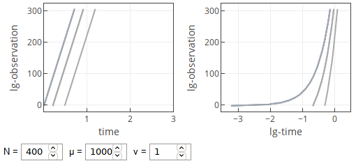
- If \( \mu \gg 1 \), then we observe exponential growth.
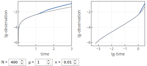
- If \( \mu \) is reasonable and \( \nu \) is small, then we observe linear growth, which transitions into squared growth for larger \( t \).
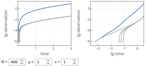
- If \( \mu \) is reasonable and \( \nu \) is moderate, then we mostly observe squared growth. For small \( t \) we may observe linear growth. Though rarely, but for large \( t \) we may observe that growth once again becomes linear.
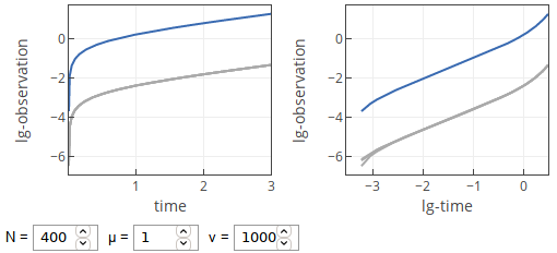
- If \( \mu \) is reasonable and \( \nu \) is large, then we will observe linear growth with transition into exponential growth.
All these regimes can be explained by Taylor series expansion of the exponential for small \( \tau \):
\begin{equation} \exp( \mu \tau ) -1 \approx \mu \tau + \mathcal{O}(\tau^2) . \end{equation}
When \( \mu \) is large, then one needs to take into account more than first order terms, so the overall shape looks like an exponential. For moderate \( mu \) in some cases one can ignore the higher order terms.
 Fig. 1:Temporal curves with large μ.
Small \( \nu \) lead to large values of \( t_i \). Most, if not all, of \( t_i \) will be larger than the small times we want to observe. Thus for small \( t \) we observe just a single exponential growth in the first spatial unit. Which is linear for \( t \ll 1 \).
 Fig. 2:Temporal curves with small ν.
With moderate \( \nu \) significant number of \( t_i \) will be within the range of small times we want to observe. So the observed dynamics will be a sum of linear growths, which are reasonably well spread out. Integral of a linear function is a squared function. Therefore we observe squared growth.
 Fig. 3:Temporal curves with moderate ν.
With large \( \nu \) many of \( t_i \) will be very small and practically indistinguishable from our perspective. Thus the sum would be well described by an exponential function, which for \( t \ll 1 \) is well approximated by linear function.
 Fig. 4:Temporal curves with large ν.
Interactive app
Feel free to explore these intuitions using the interactive app below. This app provides two plots, which show the same data, but the left one uses log-linear axes, while the right one uses log-log axes. Blue curves correspond to the global dynamics (sum of the local dynamics), while gray curves show example curves of the local dynamics.
