Space and time symmetry in the compartmental voter model
Today we continue our series of posts on compartmental voter model. Today we ask a question: is there a symmetry between stationary (temporal) and spatial distributions? Note that we have observed this symmetry in the infinite capacity case, but we haven't yet looked from this perspective in the finite capacity case. In this case we just know that we no longer observe the Beta distributions, which we have observed in the infinite capacity case.
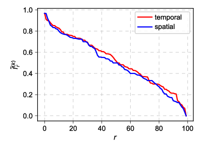
In the last post we have looked at the finite capacity case when the number of compartments, \( M \), is small. We have mentioned that in this case spatial rank-size distributions would be not very informative. Now let us consider larger \( M \) and make a comparison between the spatial rank-size distribution and the temporal rank-size distribution. Given some time for the temporal distribution converge, we should see that both rank-size distributions are quite similar.
 Fig. 1:Temporal (red) vs spatial (blue) rank-size distribution: N=2600, T=2, M=100, C=30, ε=2.
Note that in the figure above we study \( f \) instead of the usual \( X \). While \( X \) stands for the total population of certain agent type in certain compartment, \( f \) corresponds to the fraction of agents of certain type in certain compartment:
\begin{equation} f_i^{(k)} = \frac{X_i^{(k)}}{N_i}, \qquad \text{if} \quad \; N_i > 0 . \end{equation}
This fraction is somewhat nicer observable, because in the empirical data we often have compartments of very different sizes (e.g., the sizes of the polling stations in the Lithuanian parliamentary election data vary over almost two degrees of magnitude) and thus making comparisons in absolute numbers will often not make very much sense.
Furthermore the compartmental voter model, with certain parameter sets at least, seems to generate rather broad distributions of the total number of agents in the compartment, \( N_i \). Therefore the population fraction is nice observable for our model, too.
The not so nice thing about the population fraction is that we could, in theory, end up with division by zero. We resolve this issue by replacing those cases with zeros:
\begin{equation} f_i = 0 , \quad \text{if} N_i=0 . \end{equation}
Interactive app
Once again the app is quite similar to the one in the original post. The main differences are that we have two agent types (which are assumed to be statistically indistinguishable) and a different observable. Also in this app we report only the rank-size distributions: red dots correspond to the temporal (stationary) distribution, blue dots correspond to the spatial distribution.

Acknowledgment. This post is based on research which was carried out as a part of the postdoctoral fellowship ''Physical modeling of order-book and opinion dynamics'' (09.3.3-LMT-K-712-02-0026) project. The fellowship is funded by the European Social Fund under the No 09.3.3-LMT-K-712 ''Development of Competences of Scientists, other Researchers and Students through Practical Research Activities'' measure.
