Compartmental voter model with finite capacity

In the last post we have introduced you to the compartmental voter model [1]. While we have introduced the concept of capacity and allowed for a brief exploration of it, this time we dig slightly deeper into this topic.

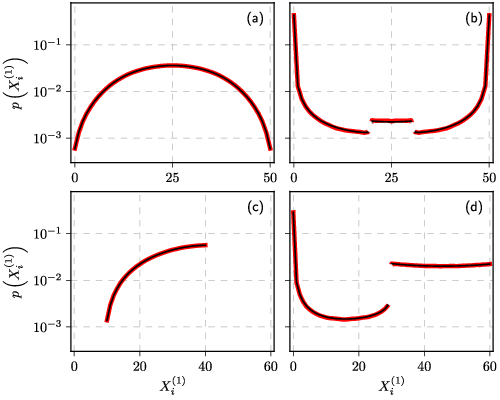
Note that if the capacity is finite, we are no longer able to obtain close form result. Yet we can rely on the fact that our model is in fact a Markov chain. Thus we can obtain the stationary distribution by solving eigenproblem for the transition matrix. While this is doable, it is extremely impractical as the effective number of system states grows extremely fast with \( M \) and \( T \). Thus we can obtain, in reasonable time, results for small values of \( M \) and \( T \). While \( N \) can be larger, but it still should not be extremely big. Note, that stationary distribution we have obtained in certain cases posses discontinuous jumps.

Fig. 1:Model (red) vs MC result (black) for finite capacity: N=100, M=2 and T=2 ((a) and (b)), N=90, M=3 and T=1 ((c) and (d)), C=40 (c), 60 ((a) and (d)) and 80 (b), ε=2 ((a) and (c)) and 0.03 ((b) and (d)).

Note that here we report only stationary distributions via probability density functions. This is because with low \( M \) spatial rank-size distribution plot is somewhat uninformative as one can have at most \( M \) points in those plots.

Interactive app

The app we make available with this post is quite similar to the one from the earlier post, but there are some important differences. Notably this app allows for different values of \( T \) and \( M \). Though to allow for this we have imposed another restriction: you can input just one value of \( \varepsilon \), which is assumed to be the same for all agent types. This effectively means that different agents types are statistically indistinguishable as all relevant characteristics are the same.

So, this time feel free to explore the implications of finite capacity with low \( T \) and \( M \). Note that with \( \varepsilon < 1 \) you are likely to observe discontinuous distributions of \( X \).

Acknowledgment. This post is based on research which was carried out as a part of the postdoctoral fellowship ''Physical modeling of order-book and opinion dynamics'' (09.3.3-LMT-K-712-02-0026) project. The fellowship is funded by the European Social Fund under the No 09.3.3-LMT-K-712 ''Development of Competences of Scientists, other Researchers and Students through Practical Research Activities'' measure.

References

• A. Kononovicius. Compartmental voter model. Journal of Statistical Mechanics 2019: 103402 (2019). doi: 10.1088/1742-5468/ab409b. arXiv: 1906.01842 [physics.soc-ph].