Compartmental voter model

In sociological papers it is quite common to see the analysis of how specific socio-demographic factors influence voting behavior. In opinion dynamics on the other hand we are usually interested only in contagion effects. Though some of the models sometimes are more sophisticated and include things like bounded confidence, explicit or implicit (like in Ishii's trust and suspicion models we have recently discussed) network structure, which effectively segment the society into separate groups. Yet these groups are surely not equivalent to the socio-demographic groups.

Another issue is that often in opinion dynamics the data is not temporal, but is spatial instead. One way to avoid this problem is to assume that electoral districts (our spatial dimension) are independent of each other (we have implicitly made this assumption here). Though obviously, this assumption is not true. If you recall another recent post, then you likely already know what we will do here. We will discuss an extension of the voter model, which is similar to the discussed Kawasaki's idea about the Ising model.

Note that the model in question was published in [1]. This post reuses some of the figures present in the paper.

The model

We will assume that there are \( N \) agents, each of which is in one of \( T \) states. These states can correspond to opinions or to socio-demographic types (hence the notation). Similarly to the spins in the Kawasaki's Ising model, the states of the agents in this model are also assumed to be fixed. Instead the agents are able to move between \( M \) compartments as long as the compartments are not overcrowded (they are assume to have inherent capacity \( C \)).

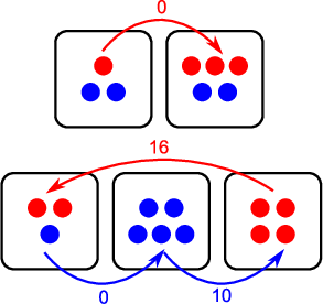
Let us assume that the movements between compartments are based on homophily. With the actual rule inspired by the original voter model. Given different source and destination compartments, \( i \neq j \), and that the destination compartment is not over its capacity, \( N_j < C \), the transition rate is assumed to be:

\begin{equation} \lambda_{\left(k\right)}^{i\rightarrow j} = X_{i}^{\left(k\right)}\left(\varepsilon^{\left(k\right)}+X_{j}^{\left(k\right)}\right) . \end{equation}

Otherwise the transition rate is equal to zero. In the above \( X_i^{(k)} \) is the number of type \( k \) agents in the district \( i \), \( \varepsilon^{(k)} \) is the individual transition rate for type \( k \), \( N_j \) is total number of agents in the district \( j \).

Fig 1.Schema of the compartmental voter model. Arrows show directions of possible transitions along with respective transition rates. Note that zero rate means that this transitions will not happen unless something changes. Parameters: N = 20, T=2, M=5, C=5, ε=2.

Note that the compartmental voter model is conceptually similar to the original Schelling's model as well. Yet we implement a continuous transition rule instead of discrete one. This allows us to implement the compartmental voter model in continuous time.

Dynamics

Sadly, the model can be studied analytically only if the capacity is effectively infinite, \( C = N \). If so, then we can write total entry and exit rates for the compartments. Otherwise, if \( C < N \), the total entry and exit rates do not have closed forms. Furthermore the analytical results apply only to the stationary probability density functions and not to the compartmental rank-size distributions in which we are interested in.

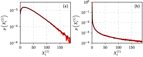
For the infinite capacity case it can be easily shown that the stationary distribution is Beta distribution, or for finite \( N \) it is Beta-binomial distribution instead.

Fig 2.Model (red) vs Beta-fit (black): N=3000, T=1, M=100 and C=N (both), ε=2 (a) and 0.03 (b).

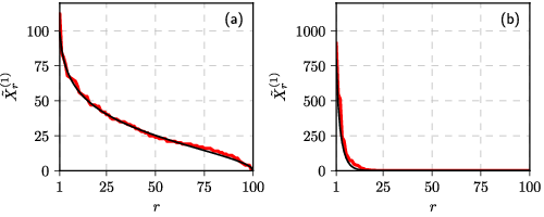
Yet interestingly the same fit also applies to the compartmental rank-size distribution.

Fig 3.Model (red) vs Beta-fit (black) with the same parameters as in the previous figure

Note that there is an essential difference between how we calculate stationary and compartmental distributions. Stationary distributions are obtained by observing the model over time at fixed spatial unit (as the model is ergodic, this approach is equivalent to observing an ensemble), while compartmental distributions are obtained by observing the model over space at fixed time. They do not need to match, yet they do.

Interactive app

Meanwhile we invite you to explore interactive app, which implements the compartmental voter model. Though there are few restrictions.

First of all note that in this app has fixed \( T \) to be \( 1 \). Allowing for a flexible number of the agent types would make user interface more complex than it is currently necessary. Having \( T>1 \) does somewhat change dynamics of the model, but only if \( C < N \). Because different agent types interact only via finite capacity.

Also we have fixed \( M \) to be \( 100 \). While this choice is not that necessary, but it doesn't limit the user a lot as \( M \) doesn't have huge impact on the observed dynamics of the model. Having it at \( 100 \) is optimal, because the simulation is still not that resource intensive, but we can also see pattern in the rank-size distribution.

Note that in this app you specify not the total number of agents, \( N \), but \( X_i(0) \), which corresponds to the number of agents in any given compartment \( i \) at time \( t = 0 \). Therefore initial spatial distribution of the agents is uniform over compartments.

Note that if \( C < N_i(0) \cdot M \), you can change the fitting parameters, \( \alpha \) and \( \beta \). Otherwise they are set automatically to values obtained during analytical derivation of the stationary distribution.

Finally, allow some time for the stationary distribution, which is obtained from the first compartment time series, to converge. It does take some time as well as enough data points are needed for the probability density function to start look smoother.

So feel free to explore the model using the app below. Note that in a few weeks time, with new posts on this same model, we will add a few apps more.

Acknowledgment. This post is based on research which was carried out as a part of the postdoctoral fellowship ''Physical modeling of order-book and opinion dynamics'' (09.3.3-LMT-K-712-02-0026) project. The fellowship is funded by the European Social Fund under the No 09.3.3-LMT-K-712 ''Development of Competences of Scientists, other Researchers and Students through Practical Research Activities'' measure.

References

• A. Kononovicius. Compartmental voter model. Journal of Statistical Mechanics 2019: 103402 (2019). doi: 10.1088/1742-5468/ab409b. arXiv: 1906.01842 [physics.soc-ph].