Stationary distribution of the poll-delayed voter model

In the last few posts, I have introduced you to two variations of the voter model enhanced with polling mechanism [1]. These two variations differed in whether the announcement of poll outcome is delayed or not. This time, we will explore the distributions obtained from these models.

Temporal evolution of ensemble PMFs

Typically, we are interested in the stationary distributions generated by the models, as we would expect these to be compared against the empirical data. While this approach might be wrong (see posts on compartmental voter model) in a sense that the data is spatial and has inherent spatial correlations. Nevertheless, it is still a valuable tool in understanding the effects various mechanisms might have.

The interactive app in this post determines the stationary distributions by simulating ensembles (collections of model instances that evolve under the same parameters and start from the same initial conditions) over time. Each frame you see in the app is a snapshot of the order parameter value distribution across multiple simulated instances (\( 10^3 \) for each model) at a fixed time point (given in the label above the plot).

Initially, the probability mass function (abbr. PMF) over the ensembles will be relatively narrow and concentrated around the initial condition. As time passes, the ensemble PMFs will spread out (their variance will grow). At a certain, the variance growth will settle down, and the model will reach stationary PMF. However, the exact shape in which stationary PMF settles depends on the polling period as well.

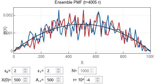
If the polling period is short, the PMFs of both models will approach the dark gray curve. The dark gray curve shows beta-binomial PMF, representing stationary distribution expected to be obtained from the standard noisy voter model with the same \( \varepsilon_i \) parameter values. For longer polling periods, the shape of the stationary distribution will be different.

Fig. 1:Ensemble PMF of both models (red - with delay, blue - without) after large number of polls when polling period is short. Dark gray curve shows stationary PMF expected from the standard noisy voter model with the same parameters.

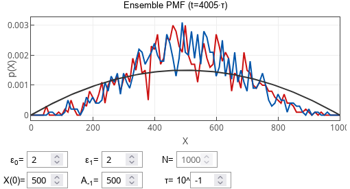
Both models will have the same (or at least very similar-looking) stationary PMFs for very long polling periods. Longer polling periods allow the simulated system to incorporate previous poll information fully. One might say that the simulated system manages to catch up to the most recent information.

Fig. 2:Ensemble PMF of both models (red - with delay, blue - without) after large number of polls when polling period is long. Notice that both red and blue curves have similar shape and are narrower than the gray curve.

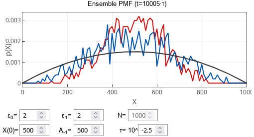
The interesting thing happens for intermediate polling periods. The model curves are different! The stationary PMF of the model with delays for the intermediate polling periods is narrower (with a lower variance) than the model without delays. I find it hard to comprehend the physical reason why this happens, but it follows from the Yule-Walker equations, which we will cover in a later post.

Fig. 3:Ensemble PMF of both models (red - with delay, blue - without) after large number of polls when polling period is intermediate. Notice the minor, yet noticeable, difference between the red and blue curves.

Interactive app

At this point, we invite you to check the insights using the interactive app below. One interesting the to check would be to make \( X(0) \) and \( A_{-1} \) different. This change will not affect the ensemble PMF of the model with no delays (blue curve). In contrast, the ensemble PMF of the model with delays (red curve) will jump around initially (as long as the simulated instances are strongly cross-correlated).

References

• A. Kononovicius, R. Astrauskas, M. Radavičius, F. Ivanauskas. Delayed interactions in the noisy voter model through the periodic polling mechanism. Physica A 652: 130062 (2024). doi: 10.1016/j.physa.2024.130062. arXiv:2403.10277 [physics.soc-ph].