Supportive interactions in the noisy voter model

Typically voter models assume that recruitment occurs between two interacting individuals. Obviously recruitment can occur only if these individuals have different opinions. While nothing will happen if these individuals hold the same opinions. Though Latane social impact [1] predicts that support provided by like-minded individuals can also play a role. In this post I'll discuss my last work done during my postdoctoral project [2], which introduces supportive interactions into the voter model.

The model

Let the agent in the same state provide support to each other and thus discourage switching away from the current state. First we will assume that this support discourages both independent and imitative transitions:

\begin{equation} \lambda^{+} \left(X\right)=\left(N-X\right)\left[\sigma_{1}+\frac{h}{N^{\alpha}}X-\frac{q}{N^{\beta}}\left(N-X\right)\right]_{+}, \end{equation}

\begin{equation} \lambda^{-} \left(X\right)=X\left[\sigma_{0}+\frac{h}{N^{\alpha}}\left(N-X\right)-\frac{q}{N^{\beta}}X\right]_{+}. \end{equation}

These are mostly the usual transition rates of the noisy voter model with \( \sigma_i \) standing for independent transition rates, \( h \) representing recruitment (herding) rate, \( X \) corresponding to the number of agents in the first state and \( N \) being total number of agents. If \( \alpha = 0 \), then the noisy voter model would be non-extensive (has broad stationary distribution for any \( N \)). While for \( \alpha = 1 \) the model is extensive (has narrow stationary distribution, which shrinks as \( N \rightarrow \infty \).

The above rates are different from the usual transition rates due to the third term in the square brackets, which describes interaction with like-minded peers. Two new parameters control the interaction: \( q \) is the supportive interaction rate, while \( \beta \) has the same meaning as \( \alpha \), but applies only to supportive interactions. As you can see this interaction decreases the respective transition rate. These rates make sense only if they are non-negative, so we have to assign the square brackets a special meaning:

\begin{equation} \left[z\right]_{+}=\max\left(z,0\right). \end{equation}

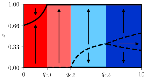
Purely from examining the transition rates it is clear that the model will posses four distinct phases (three if \( \sigma_0 = \sigma_1 \)):

• In the first phase both rates are positive for all \( X \). In this phase this model is equivalent to the noisy voter model with appropriately adjusted parameter values. This phase is observed if \( q < N^{\beta-1} \min\left(\sigma_0, \sigma_1\right) \).
• In the second phase one of the rates would become negative, if not for the brackets, and the effects of the supportive interactions become more visible. Namely, the system is being quickly pushed towards consensus surrounding the more "attractive" state (one associated with larger \( \sigma_i \)). This phase is observed if \( q < N^{\beta-1} \max\left(\sigma_0, \sigma_1\right) \).
• In the third phase both of the rates would become negative, if not for the brackets. This phase is characterized by three stationary points, with the two consensuses being stable and the intermediate state being unstable. This phase is observed if \( q < N^{\beta-\alpha-1} \left(N h+N^{\alpha}\left(\sigma_{0}+ \sigma_{1}\right)\right) \).
• In the fourth phase for certain values of \( X \) both of the transition rates would be negative, if not for the brackets. If you start at such \( X \), then the system would remain at \( X \). This phase is observed if \( q \geq N^{\beta-\alpha-1} \left(N h+N^{\alpha}\left(\sigma_{0}+ \sigma_{1}\right)\right) \).

An example of a bifurcation diagram of the model, with all 4 phases visible, is given below. While bifurcation diagram retains its qualitative behavior, but it slightly varies with \( \alpha \) and \( \beta \). Most notably with \( \alpha = 0 \) the first phase is characterized by a stationary distribution, which is Beta distribution. Also some of the critical points, ones separating the distinct phases, either go to zero or diverge towards infinity as \( N \rightarrow \infty \). This means that in certain scenarios not all phases will be observable. For a more complete picture of the phase behavior of the model see Fig. 2 in [2].

Fig 1.Bifurcation diagram of the model with α=β=1 (corresponds to Fig. 2 (a) from the article).

Interactive app

Use the app below to explore the four phases of the noisy voter model with supportive interactions. This app shows you two plots: time series plot (on the left) and rate plot (right). Time series plot show \( 10 \) sample trajectories, so that you could where different trajectories tend to. Rate plot shows to curves, red curve corresponds to death rate, while green curve corresponds to birth rate. Rate plot allows to anticipate where the stationary points will be and whether they will be stable. In most cases the model will converge towards stable stationary points, so we neglect the usual statistical analysis.

Acknowledgment. This post was written while reviewing literature relevant to the planned activities in postdoctoral fellowship ''Physical modeling of order-book and opinion dynamics'' (09.3.3-LMT-K-712-02-0026) project. The fellowship is funded by the European Social Fund under the No 09.3.3-LMT-K-712 ''Development of Competences of Scientists, other Researchers and Students through Practical Research Activities'' measure.

References

• B. Latane. The psychology of social impact. American Psychologist 36: 343-356 (1981). doi: 10.1037/0003-066X.36.4.343.
• A. Kononovicius. Supportive interactions in the noisy voter model. Chaos, Solitons and Fractals 141: 110627 (2021). doi: 10.1016/j.chaos.2020.110627. arXiv:2001.11066 [physics.soc-ph].