Waiting time paradox

Last time we have introduced a concept of waiting time. We have assumed that some time has passed since the last event and wanted to how long do we have to wait until another event. The time since the last event was a thing we knew. Now let us consider a slightly different case - what happens when we do not know when the last event happened, how long do we have to wait until the next event?

In other words, imagine you just have come to a bus stop. If you know that the average bus interarrival time is \( 15 \) minutes, then how long would you expect to have to wait? Straightforward answer seems to be \( 7.5 \) minutes, but is it a correct answer?

Perfectly reliable buses

Actually, we did not provide a crucial piece of information - how reliable the buses are. If the buses are perfectly reliable, then the answer is indeed \( 7.5 \) minutes:

\begin{equation} \langle w \rangle = \int_0^{\langle\tau\rangle} w \cdot \frac{1}{\langle\tau\rangle} dw = \frac{\langle\tau\rangle}{2} . \end{equation}

In the above \( \langle\tau\rangle \) is the average bus interarrival time, which in our case it is \( 15 \) minutes. The above expression implicitly assumes that we are equally likely to come to the bus stop at any point between the bus arrivals.

Imperfect buses

Now let us assume that sometimes buses might not be that perfect. Let them come any time (equally likely) within \( \Delta \) minutes of the scheduled time (they are not allowed to arrive earlier than buses scheduled before them). At first the imperfection doesn't seem to have an effect, because shorter inter-event times are as likely to appear during the day as the longer inter-event times. Actually, inter-event time follows triangular distribution:

\begin{equation} p(\tau)= \begin{cases} \frac{2 \Delta+\tau-\langle \tau\rangle }{4 \Delta^{2}} & \langle \tau\rangle - 2 \Delta\leq\tau\leq\langle \tau\rangle ,\\ \frac{2 \Delta+\langle \tau\rangle -\tau}{4 \Delta^{2}} & \langle \tau\rangle \leq\tau\leq\langle \tau\rangle + 2 \Delta,\\ 0 & \text{othewise}. \end{cases} \end{equation}

But this distribution is at odds with how we as observers experience inter-event times when we start the observation at a random time and wait for the next event to happen.

Let us imagine simpler case first, with \( 50 \% \) probability inter-event time is \( 5 \) minutes, and otherwise it is \( 15 \) minutes. Both inter-event times are equally likely, but if we start waiting at a random time, we are three times as likely to start it during the \( 15 \) minute break. To account for this we need to weight the distribution according to the duration of inter-event time:

\begin{equation} p\left(\tau_{o}\right)= \begin{cases} \frac{\tau_{o}}{\left\langle \tau\right\rangle }\times\frac{2 \Delta+\tau_{o}-\left\langle \tau\right\rangle }{4 \Delta^{2}} & \left\langle \tau\right\rangle - 2 \Delta\leq\tau_{o}\leq\left\langle \tau\right\rangle ,\\ \frac{\tau_{o}}{\left\langle \tau\right\rangle }\times\frac{2 \Delta+\left\langle \tau\right\rangle -\tau_{o}}{4 \Delta^{2}} & \left\langle \tau\right\rangle \leq\tau_{o}\leq\left\langle \tau\right\rangle + 2 \Delta,\\ 0 & \text{otherwise}. \end{cases} \end{equation}

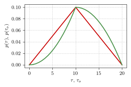
In the above \( \tau_{o} \) stands for the inter-event duration during which we start waiting for the next event. Notably the larger the \( \Delta \) the more different the distributions of \( \tau \) and \( \tau_o \) are. Comparison between the respective probability density functions is given in the figure below.

Fig 1.Comparison of interarrival time PDF (red curve) and observed interarrival time PDF (green curve).

Now the average waiting time will be given by (assuming that \( \tau \geq 2 \Delta \)):

\begin{equation} \langle w \rangle = \frac{\langle\tau_o\rangle}{2} = \frac{2 \Delta^2 + 3 \langle\tau\rangle^2}{6 \langle\tau\rangle} . \end{equation}

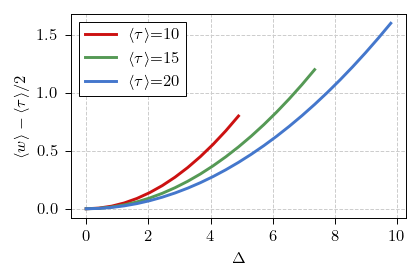
If we have \( \tau < 2 \Delta \), and you can explore this range of parameters using the app below, then the case becomes much more complicated. I will skip analytical analysis of the particular range of parameters, but you can still explore it numerically, and see that general conclusion still holds - you always wait longer than you would expect by halving the mean interarrival time.

Fig 2.Difference between the mean waiting time and the half of the mean interarrival time

Interactive app

Using the app below you can explore this problem from the numerical simulation point of view. Observe that your average waiting time is always longer than in the ideal case when buses are never late.

The upper plot in this app shows the simulated series. The app generates 12 hour long series and then picks one random time to start waiting for the next event (arrival). Events are scheduled each \( \langle\tau\rangle \) minutes, but may deviate (be early or late) from the scheduled time by \( \Delta \) minutes. In the upper plot blue spikes correspond to the arrival events and the singular red spike corresponds to the start of the observation (you arriving to the bus stop).

The bottom plot shows the probability density function of the waiting time, when the observation is started at a random time.