Fermi-Dirac statistics with single conduction level

Have you ever wondered how Fermi-Dirac statistics arises? I may have wondered during my bachelor degree studies, but now I only remember derivation done by the means of combinatorics. In this post I continue my wandering from a perspective of numerical simulation of a highly simplified system.

In the previous post we have built a model in which particles may freely jump between the energy levels (restricted only by the Pauli exclusion principle and Boltzmann statistics). This is not necessarily possible in real life systems. In semiconductors individual traps may have a single characteristic trap depth, or multiple depths which would not span full spectrum of available trap depths. In such case we need to assume existence of a conduction band energy level, which allows particles to travel between different traps.

Let us examine this particular case in this post.

Model

1. Let the system be composed of \( 100 \) energy levels. The highest level is special (for the reason obvious from further assumptions) and is referred to as the conduction level.
2. Each energy level has energy equal to its index. In other words \( E_i = i \) with \( i = 1, 2, \ldots, 100 \).
3. Let there be \( 50 \) particles.
4. Particle may jump to an energy level if it is empty. Namely, single particle can occupy single energy level.
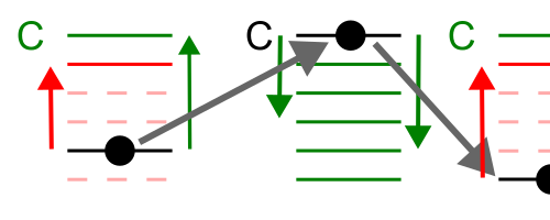
5. Particle occupying the highest (conduction) level may jump to any trap level with probability given by the Boltzmann factor.
6. Particle occupying any lower (trap) level may jump only to the conduction level with the probability given by the Boltzmann factor.

Fig 1.Schematic depiction of a series of consecutive jump in the considered model. Main thing to notice is that jumps from deep (trap) levels are allowed only to the conduction level. From the conduction level any other deeper layer can be reached.

Boltzmann factor is given by:

\begin{equation} P_{i \rightarrow j} = \min\left[1, \exp\left( \frac{E_i - E_j}{k_B T} \right) \right]. \end{equation}

Because conduction level is the highest energy level, probability to jump "down" (i.e., \( C \rightarrow j \)) from it is always \( 1 \). Escaping the trap on the other hand takes significant amount of time as jump "up" (i.e., \(j \rightarrow C \)) probability will be relatively small.

Interactive app

All is fine and interesting, but we would like to have average occupation of the energy levels to follow Fermi-Dirac distribution function:

\begin{equation} F\left(E_i\right) = \frac{1-{\bar n}_{\text{free}}}{1+\exp\left(\frac{E_i - E_F}{k_B T}\right)} . \end{equation}

In the above \( E_F \) is Fermi energy, which marks the inflection point of the distribution. While \( {\bar n}_{\text{free}} \) stands for the density of free particles. So, does Fermi-Dirac distribution still apply to this scenario? Check it yourself using the app below (black curve represents \( F\left(E\right) \) from the above).

Please note, that it takes much more time for the numerical results to converge towards the theoretical curve (at least in comparison with the previous post). This is because detrapping to the conduction level is quite problematic and this hampers overall particle mobility over the energy levels.