Waiting time distribution

Last time we have seen that interarrival (or, more generally, inter-event) times in the Poisson process follow exponential distribution. Inter-event times tell us how much time has passed since the last event, but we are often also interested in times till event given that \( T \) time has passed since previous event.

In the terms of the original problem we could ask the question: what is the expected time for the next student to come? Let us assume that \( 5 \) minutes has passed since the arrival of the last student. Let us recall that \( 4 \) students arrive per hour (meaning on average \( 15 \) minutes between them). Intuitive and wrong answer would be \( 10 \) minutes.

Waiting time distribution of the Poisson process

Why \( 10 \) minutes is wrong answer should be clear from the microscopic model of the Poisson process: there is fixed probability for an event to occur during each time step. This probability doesn't depend on anything but the time scale. This mean that for the Poisson process:

\begin{equation} p \left( \tau | T \right) = p( \tau ) = \lambda \exp\left(- \lambda \tau\right). \end{equation}

Implying that the expected time is \( \frac{1}{\lambda} \).

Another way to obtain the same intuition is to look at the survival function of the exponential distribution:

\begin{equation} P(X > t) = \exp(-\lambda t). \end{equation}

If we are stating that until time \( T \) no event has happened, we are effectively ignoring all events that could have happened in that time. We are interested in survival from time \( T \) onwards, so we simply rescale the survival function, so that it would be equal unity at time \( T \). In case of the exponential distribution:

\begin{equation} P(X > t > T) = \exp(-\lambda t) \cdot \exp(\lambda T) = \exp\left[-\lambda \cdot (t-T)\right]. \end{equation}

Recalling that we care about the distribution of \( \tau = t-T \), we see that it is distributed exactly the same as the inter-event time.

Survival function of the uniform distribution

Survival function of the uniform distribution (let the interval of possible values be \( [ 0, 2 \langle\tau\rangle ] \)) is given by:

\begin{equation} P(X > t) = 1 - \frac{t}{2\langle\tau\rangle} . \end{equation}

If we have waited for \( T \) until the event (let \( T < 2 \langle\tau\rangle \)), then the survival function:

\begin{equation} P(X > t > T) = \frac{2\langle\tau\rangle - t}{2\langle\tau\rangle - T} = \frac{2\langle\tau\rangle - T - (t-T)}{2\langle\tau\rangle - T} . \end{equation}

Recalling that we care about the distribution of \( \tau = t-T \), we see that it is distributed almost the same as the inter-event time. Distribution appears to remain uniform distribution, but the interval of possible values has shrunk to \( [ 0, 2 \langle\tau\rangle - T ] \).

Survival function of the normal distribution

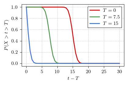
Survival function of the normal distribution (let \( \sigma = 1 \)):

\begin{equation} P(X > t) = \frac{1}{2} \left[ 1 - \operatorname{erf}\left(\frac{t - \langle\tau\rangle}{\sqrt{2}}\right) \right] . \end{equation}

Now the error function, \( \operatorname{erf} \), is a rather complicated thing. We won't be able to do the same analytical exploration we did with the exponential distribution or the uniform distribution survival functions. But the core idea would be that \( P(X > T) \) is just a constant, which scales the survival function:

\begin{equation} P(X > t > T) = \frac{1}{P(X > T)} \cdot P(X > t). \end{equation}

When we consider survival of \( \tau = t - T \) we simply shift the survival function to the left. For the exponential distribution such shift doesn't change anything, because exponential function has translation symmetry (it doesn't experience any ageing effects - the mean waiting time is the same as the mean interarrival time). Other distributions, such as the normal distribution, do not have this symmetry and thus exhibit ageing effects - the mean waiting time is always smaller than the mean interarrival time.

Fig 1.Survival functions of the normal distribution.

Interactive app

Use the app below to explore the waiting time distribution. You can choose time duration you have already waited for \( T \), the mean of the interarrival distribution \( \langle\tau\rangle \) and the interarrival distribution itself. Note that for the normal and uniform distributions setting \( T > \langle\tau\rangle \) may not make much sense, but otherwise feel free to explore! Note that the red curve corresponds to the interarrival time distribution (its PDF), while blue curve represents waiting time distribution (its PDF).