Analytical solution of the boring basketball game

FiveThirtyEight has an interesting column, Riddler column, which I follow with great interest. In this post we will revisit boring basketball game problem from analytical perspective. Though we will cheat a bit and use Python to do the algebra for us.

Analysis of the problem

The problem appears to be symmetric only from a first glance. It is actually asymmetric. To see this let us analyze a few sample cases.

First let us take a look at first and second possession. It is easier to look at pairs of possessions, because every pair starts and ends exactly the same way (the ball starts in the same hands). In fact further analysis applies to any other pair of possessions (there is no time dependence in the schema) as long as initial score difference is zero.

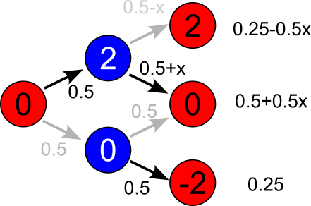
Fig 1.Case when initial difference in score is zero. Circles represent states (colored based on the team possessing the ball) reachable via transitions. These are represented by darker (made the shot) and lighter (missed the shot) arrows.

As we can see in the schema above during the possession by the red team there is an equal chance for two outcomes: red team makes the shot (difference becomes \( 2 \)) and they miss (difference remains unchanged).

If the red team makes a shot, then blue team gets possession with score difference being \( 2 \). As the blue team is now trailing, it attains losers advantage: its probability to make the shot is \( 0.5 +x \).

If the red team misses a shot, then blue team gets possession with score being equal. In this case blue team doesn't get the losers advantage and has equal chances to make the shot or miss.

Calculating the probabilities of the score difference before the third possession (outcome of the two possessions prior) is a trivial matter. As we can see the probability for the score difference to be negative (to be in favor of the blue team) is higher than the probability for the score difference to be positive. Hence, it is obvious that blue team has certain advantage.

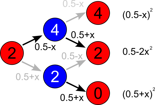
Fig 2.Case when initial difference in score is positive.

As we can see in the schema above whenever score difference is positive (schema considers case when difference is \( 2 \), but you can simply add any even number to all numbers in the schema and end up with the same outcome probabilities), there will be a slight drift towards equal score.

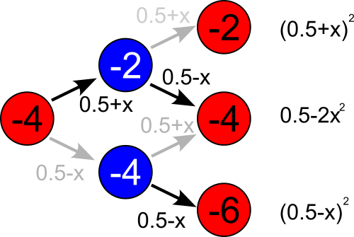
Fig 3.Case when initial difference in score is negative (-4 or larger).

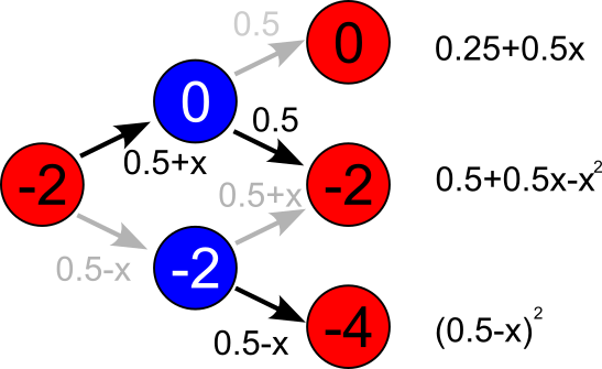
Drift towards zero is also observed when initial score difference is negative. Yet notice that the schema above only applies for differences of \( -4 \) or larger (in a sense that difference of \( -16 \) is larger than \( -4 \)), as if we add \( 2 \) to the numbers then the outcome probabilities change (see below).

Fig 4.Case which breaks symmetry between negative and positive score differences.

Exactly because of this last case, the blue team has a considerable advantage.

Solution

As we now know the probabilities of all possible outcomes, we can build a transition matrix and use linear algebra tools to calculate the system state (score difference) after \( 200 \) possessions. The problem is that the transition matrix is kind of large.

Let us use Python to do the heavy lifting! Let us also use our numerical discovery (from the previous post) that \( x \approx 0.25 \).

import numpy as np

# configurable parameters
x = 0.25
possessions = 100  # <= 100

assert possessions <= 100, "Transition matrix size needs to be adjusted manually"

# creating and filling in transition matrix
transition_matrix = np.zeros((201, 201))

# transitions from score difference of zero
transition_matrix[101, 100] = 0.25  # difference becomes -2
transition_matrix[101, 101] = 0.5 + 0.5 * x  # difference remains 0
transition_matrix[101, 102] = 0.25 - 0.5 * x  # difference becomes 2

# transitions from score difference of -2
transition_matrix[100, 99] = (0.5 - x) ** 2  # difference becomes -4
transition_matrix[100, 100] = 0.5 + 0.5 * x - x**2  # difference remains -2
transition_matrix[100, 101] = 0.25 + 0.5 * x  # difference becomes 0

# other negative cases
for idx in np.arange(0, 100):
    # to higher
    transition_matrix[idx, idx + 1] = (0.5 + x) ** 2
    # to lower
    if idx > 0:
        transition_matrix[idx, idx - 1] = (0.5 - x) ** 2
    # stay
    transition_matrix[idx, idx] = 0.5 - 2 * (x**2)

# all positive cases
for idx in np.arange(102, 201):
    # to lower
    transition_matrix[idx, idx - 1] = (0.5 + x) ** 2
    # to higher
    if idx < 200:
        transition_matrix[idx, idx + 1] = (0.5 - x) ** 2
    # stay
    transition_matrix[idx, idx] = 0.5 - 2 * (x**2)

# initial state
state = np.zeros(201)
state[101] = 1  # all games start from score difference of zero

# play the games analytically
tm = np.linalg.matrix_power(transition_matrix, possessions)
fin_state = np.matmul(state, tm)

# output the results
print(f"p(draw) = {fin_state[101]:.4f}")
print(f"p(red)  = {np.sum(fin_state[102:]):.4f}")
print(f"p(blue) = {np.sum(fin_state[:101]):.4f}")

> python boring-game.py
p(draw) = 0.5000
p(red)  = 0.1250
p(blue) = 0.3750

Well this is actually semi-analytical solution, because proper finding of the \( x \) could only be done with numerical root solving algorithm. I doubt whether analytical engines in Python or Mathematica would deal well with raising 200x200 matrix to the 100th power. Solving eigenproblem would likely be not as easy, too. Though I might be wrong in my pessimistic predictions.