Approximating characteristic function of bounded Pareto distribution with α=1

September 08, 2026 Aleksejus Kononovicius #statistics #power-law distributions #Python #B. Kaulakys

During the summer, I received an email from a researcher at university abroad inquiring about how we (myself and my senior colleague, prof. B. Kaulakys) derived the approximation for the characteristic function of bounded Pareto distribution (for the particular case with $ \alpha = 1 $). The approximation was given in [1], but derivation turned out to be somewhat more involved than I remembered. Originally, I derived it with the help of Wolfram Engine, while my colleague consulted various mathematical formula compendiums. Unfortunately, I was unable to find any notes containing the derivation. So I have attempted to reconstruct a combined approach from scratch. You'll find the derivation below.

Exact characteristic function

Let us consider a characteristic function of bounded Pareto distribution with $ \alpha=1 $. With $ \tau_{\text{min}}\leq\tau\leq\tau_{\text{max}} $, the probability density function of the considered distribution is given by

\begin{equation} p\left(\tau\right)=\frac{\tau_{\text{min}}\tau_{\text{max}}}{\tau_{\text{max}}-\tau_{\text{min}}}\cdot\frac{1}{\tau^{2}}. \end{equation}

Using the definition, characteristic function is given by

\begin{equation} \chi\left(f\right)=\frac{\tau_{\text{min}}\tau_{\text{max}}}{\tau_{\text{max}}-\tau_{\text{min}}}\int^{\tau_{\text{max}}}_{\tau_{\text{min}}}\frac{e^{2\pi\mathrm{i}f\tau}}{\tau^{2}}d\tau. \end{equation}

Alternatively, using $ \mathrm{Ei} \left(\ldots\right) $ special function (see Wikipedia), we can rewrite it as follows

\begin{equation} \chi\left(f \right)=\frac{\tau_{\text{min}}\tau_{\text{max}}}{\tau_{\text{max}}-\tau_{\text{min}}}\left[2\pi\mathrm{i}f\left\{ \mathrm{Ei}\left(2\pi\mathrm{i}f\tau_{\text{max}}\right)-\mathrm{Ei}\left(2\pi\mathrm{i}f\tau_{\text{min}}\right)\right\} -\frac{e^{2\pi\mathrm{i}f\tau_{\text{max}}}}{\tau_{\text{max}}}+\frac{e^{2\pi\mathrm{i}f\tau_{\text{min}}}}{\tau_{\text{min}}}\right].\label{eq:char-advanced} \end{equation}

Exponential integral are still integrals under the hood, and thus using the exact formula is somewhat problematic. Furthermore, in [1] we primarily care about approximate behavior of the characteristic function for small $ f $. We would also prefer to have something simple to plugin into other, more complicated, expressions.

Side note: Deriving \eqref{eq:char-advanced}

First, let us calculate the following derivative

\begin{equation} \frac{d}{dx}\left(\frac{e^{ax}}{x}\right)=\frac{ae^{ax}}{x}-\frac{e^{ax}}{x^{2}}. \end{equation}

Rearranging the above leads to,

\begin{equation} \frac{e^{ax}}{x^{2}}=\frac{ae^{ax}}{x}-\frac{d}{dx}\left(\frac{e^{ax}}{x}\right). \end{equation}

Let us make an observation that the derivative of an exponential integral is given by

\begin{equation} \frac{d}{dx}\mathrm{Ei}\left(ax\right)=\frac{e^{ax}}{x}. \end{equation}

Thus, we have that

\begin{equation} \frac{e^{ax}}{x^{2}}=a\frac{d}{dx}\mathrm{Ei}\left(ax\right)-\frac{d}{dx}\left(\frac{e^{ax}}{x}\right). \end{equation}

We are interested in antiderivative of the above, which is simply

\begin{equation} \int\frac{e^{ax}}{x^{2}}dx=a\mathrm{Ei}\left(ax\right)-\frac{e^{ax}}{x}+\mathcal{C}. \end{equation}

To finally obtain \eqref{eq:char-advanced}, we just need to use this result to obtain the definite integral.

Approximating the exact expression

Let us continue with \eqref{eq:char-advanced}. If we assume that $ \frac{1}{\tau_{\text{max}}}\ll f $ (or alternatively $ f\tau_{\text{max}}\gg 1 $), we could do the following approximation

\begin{equation} \mathrm{Ei}\left(2\pi\mathrm{i}f\tau_{\text{max}}\right)\approx\mathrm{i}\pi. \end{equation}

Assuming that $ \tau_{\text{min}}\ll\tau_{\text{max}} $ yields

\begin{equation} \frac{\tau_{\text{min}}\tau_{\text{max}}}{\tau_{\text{max}}-\tau_{\text{min}}}\approx\frac{\tau_{\text{min}}\tau_{\text{max}}}{\tau_{\text{max}}}=\tau_{\text{min}}. \end{equation}

Also, we would have that $ \left|\frac{e^{2\pi\mathrm{i}f\tau_{\text{max}}}}{\tau_{\text{max}}}\right|\ll\left|\frac{e^{2\pi\mathrm{i}f\tau_{\text{min}}}}{\tau_{\text{min}}}\right| $, and thus

\begin{equation} -\frac{e^{2\pi\mathrm{i}f\tau_{\text{max}}}}{\tau_{\text{max}}}+\frac{e^{2\pi\mathrm{i}f\tau_{\text{min}}}}{\tau_{\text{min}}}\approx\frac{e^{2\pi\mathrm{i}f\tau_{\text{min}}}}{\tau_{\text{min}}}. \end{equation}

At this point we have,

$$\begin{align} \chi\left(f\right) & \approx\tau_{\text{min}}\left[2\pi\mathrm{i}f\left\{ \mathrm{i}\pi-\mathrm{Ei}\left(2\pi\mathrm{i}f\tau_{\text{min}}\right)\right\} +\frac{e^{2\pi\mathrm{i}f\tau_{\text{min}}}}{\tau_{\text{min}}}\right] = \nonumber\\ & =-2\pi^{2}f\tau_{\text{min}}-2\pi\mathrm{i}f\tau_{\text{min}}\mathrm{Ei}\left(2\pi\mathrm{i}f\tau_{\text{min}}\right)+e^{2\pi\mathrm{i}f\tau_{\text{min}}}. \end{align}$$

Let us proceed by taking Taylor series for small $ f $,

$$\begin{align} e^{2\pi\mathrm{i}f\tau_{\text{min}}} & \approx1+2\pi\mathrm{i}f\tau_{\text{min}}+\ldots,\\ 2\pi\mathrm{i}f\tau_{\text{min}}\mathrm{Ei}\left(2\pi\mathrm{i}f\tau_{\text{min}}\right) & \approx-\pi^{2}f\tau_{\text{min}}+2\pi\mathrm{i}f\tau_{\text{min}}\left[C_{\gamma}+\ln\left(2\pi f\tau_{\text{min}}\right)\right]+\ldots. \end{align}$$

Then,

$$ \begin{align} \chi\left(f\right) & \approx-2\pi^{2}f\tau_{\text{min}}-\left\{ -\pi^{2}f\tau_{\text{min}}+2\pi\mathrm{i}f\tau_{\text{min}}\left[C_{\gamma}+\ln\left(2\pi f\tau_{\text{min}}\right)\right]\right\} +\left[1+2\pi\mathrm{i}f\tau_{\text{min}}\right]=\nonumber \\ & =1-\pi^{2}f\tau_{\text{min}}+\left[1-C_{\gamma}-\ln\left(2\pi f\tau_{\text{min}}\right)\right]\cdot\left(2\pi\mathrm{i}f\tau_{\text{min}}\right). \end{align}$$

Which is exactly Eq. (28) from [1].

How good the approximation is?

As usual, I would like to provide you with an interactive app so you could compare exact and approximate expressions on your own. But, it seems it is rather complicated to evaluate \eqref{eq:char-advanced} using JavaScript (as I would need to implement some advanced numerical integration method to evaluate $ \mathrm{Ei} \left(\ldots\right) $).

Thus, I have generated few static images (these use $ \tau_\text{min} = 10^{-3} $ and $ \tau_\text{max} = 10^3 $ parameter values) using Python. Below you can see three figures which compare the absolute value, the real and the imaginary part of the exact expression (black curve) and the approximate expression (red curve).

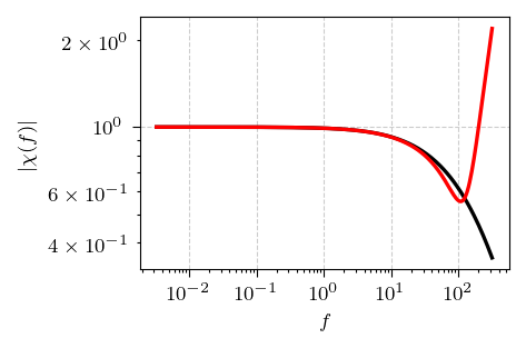Fig. 1:Comparing the absolute value of the exact expression (black curve) and the approximate expression (red curve).

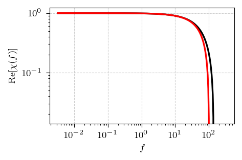Fig. 2:Comparing the real part of the exact expression (black curve) and the approximate expression (red curve).

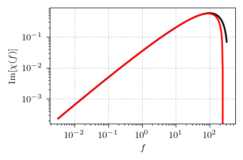Fig. 3:Comparing the imaginary part of the exact expression (black curve) and the approximate expression (red curve).

If you want to generate your own comparisons, you can reuse my Python code (which relies on mpmath library, but you could also reimplement the code using scipy.special). The figures above were generated by executing the Python code given below.

import matplotlib.pyplot as plt
import numpy as np
from mpmath import ei, euler, exp, fabs, im, log, pi, re


def exact(t_min, t_max, f):
    norm = t_min * t_max / (t_max - t_min)
    exp_max = exp(2j * pi * f * t_max) / t_max
    exp_min = exp(2j * pi * f * t_min) / t_min
    ei_max = ei(2j * pi * f * t_max)
    ei_min = ei(2j * pi * f * t_min)
    return norm * (2j * pi * f * (ei_max - ei_min) - exp_max + exp_min)


def approx(t_min, f):
    return (
        1
        - (pi**2) * f * t_min
        + (1 - euler - log(2 * pi * f * t_min)) * (2j * pi * f * t_min)
    )


t_min = 1e-3
t_max = 1e3

x_vals = np.logspace(np.log10(t_min) + 0.5, np.log10(t_max) - 0.5, num=300)
y_vals = np.array([exact(t_min, t_max, x) for x in x_vals])
y_approx = np.array([approx(t_min, x) for x in x_vals])

y_vals_im = np.array([im(y) for y in y_vals])
y_vals_re = np.array([re(y) for y in y_vals])
y_vals_abs = np.array([fabs(y) for y in y_vals])

y_approx_im = np.array([im(y) for y in y_approx])
y_approx_re = np.array([re(y) for y in y_approx])
y_approx_abs = np.array([fabs(y) for y in y_approx])

plt.figure(figsize=(3, 2))
plt.loglog()
plt.xlabel("$f$")
plt.ylabel(r"$\left|\chi(f)\right|$")
plt.plot(x_vals, y_vals_abs, "k")
plt.plot(x_vals, y_approx_abs, "r")
plt.show()

plt.figure(figsize=(3, 2))
plt.loglog()
plt.xlabel("$f$")
plt.ylabel(r"$\mathrm{Re}[\chi(f)]$")
plt.plot(x_vals, y_vals_re, "k")
plt.plot(x_vals, y_approx_re, "r")
plt.show()

plt.figure(figsize=(3, 2))
plt.loglog()
plt.xlabel("$f$")
plt.ylabel(r"$\mathrm{Im}[\chi(f)]$")
plt.plot(x_vals, y_vals_im, "k")
plt.plot(x_vals, y_approx_im, "r")
plt.show()

References

A. Kononovicius, B. Kaulakys. 1/f noise from the sequence of nonoverlapping rectangular pulses. Physical Review E 107: 034117 (2023). doi: 10.1103/PhysRevE.107.034117. arXiv:2210.11792 [cond-mat.stat-mech].