Exploring parking strategies

Traffic problems are ones we all face every day and we can explore using Physics of Risk tools such as agent-based models. Here we will take a look at a couple simple parking strategies from [1, 2].

Problem setup

Let us assume that cars arrive one at a time at rate \( \lambda \) and park in a long one dimensional parking lot. The drivers are clueless on the location of the best available parking spots, they can see just the first car parked ahead of them (and number of free spots in between them).

One can easily imagine three natural strategies [1]:

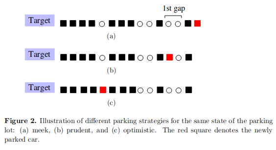
• Meek. Park at the first available spot. Just behind the last car in the parking lot. In our setup, if the last spot is taken, then the driver looks for the first gap.
• Prudent. Find the first gap and park at the left end of that gap. If there are no gaps, then you'll have to backtrack.
• Optimistic. Go all the way to the end (destination) and then backtrack until you find available spot.

These parking strategies are illustrated in the figure below. The figure and the respective caption was copied from the original article [1].

Another strategy was proposed in [2]. This strategy is known as 1/2 rule. If using this strategy, the driver ignores first \( L/2 \) spots (here \( L \) is the coordinate of the last parked car) and then acts as a prudent driver. Possibly backtracking and occupying spot at \( x > L/2 \).

While somewhat unrealistic, but we assume that only one car looks for a spot at a time. Namely, other cars are not allowed to enter the parking lot until the last entering (or leaving) car has found a spot (or left the parking lot).

We assume that a single parked car will leave at rate \( \mu \). For simplicity we set \( \mu = 1 \).

Dynamics of the model

Number of things for each of the simple strategies and the 1/2 rule can be derived analytically [1, 2]. For example, if the parking lot would be infinite, then the distribution of cars in the parking lot is Poissonian with rate parameter \( \lambda \). This means that you can reasonably expect to see \( \lambda \pm \sqrt{\lambda} \) cars in the parking lot as the model reaches stationary dynamics.

[1] also explored occupation densities for each of the simple strategies. And found that meek drivers will escape towards infinity. In our particular model meek drivers will crowd at the end of the parking lot, because if the last place is taken, then they will be looking for the first gap.

Fig 1.If meek drivers parked in the simulated parking lot.

Prudent drivers, as per [1], will leave number of available spots very close to the destination (marked by the red square), but otherwise will pack quite nicely in front of the parking lot.

Fig 2.If prudent drivers parked in the simulated parking lot.

Optimist drivers, as per [1], will quickly fill in any gap close to the destination and will pack even tighter than the prudent drivers.

Fig 3.If optimist drivers parked in the simulated parking lot.

Drivers using 1/2 rule will fill in the parking lot very much alike to prudent and optimist drivers. This strategy is superior [2] to prudent or optimistic strategy, because it gives non-vanishing probability to park at the best available spot with out backtracking. Optimistic strategy will require backtracking with probability \( \lambda / ( 1 + \lambda ) \), while ensuring parking at the best spot. Prudent strategy will rarely require backtracking, but will give the best spot with probability vanishing as \( \lambda^{-1/2} \).

Fig 4.If 1/2 rule drivers parked in the simulated parking lot.

The cost

The cost is our own addition to the model. It is calculated as follows:

\begin{equation} C_i = W x_i + D s_i . \end{equation}

In the above \( x_i \) is the parking spot coordinate (also distance to the destination, as agents are not allowed to walk over the green field), while \( s_i \) is the distance \( i \)-th driver has driven until parked at the spot. If driver parks in an optimal space \( s_i = 508 - x_i \). In the above \( W \) is the walking cost and \( D \) is the driving cost. The average cost over all currently parked cars is normalized as follows:

\begin{equation} \tilde{C} = \frac{\sum_i C_i}{\sum_{j=1}^{N} \left( W j + D \left[ 508 - j \right] \right)} = \frac{\sum_i C_i}{N \cdot \left( 508 D + \frac{W - D}{2} \cdot [N-1] \right)} \end{equation}

Denominator is effectively the total cost for all cars if they would have been parked closest to the destination.

Interactive app

This interactive app visualizes finite (508 places) one-dimensional parking lot. Empty parking spaces are shown in light gray, while taken parking space are shown in dark gray. Note that the parking lot snakes through out the green field, entrance is on the bottom left, while the destination square in on the top left (red square).

Along with visual representation of the current occupation of the parking lot two plots are shown. The first plot shows how the total number of cars (blue curve) and the position of the last parked car (dark curve) changes in time. The second plot shows normalized average cost for all currently parked cars.

References

• P. L. Krapivsky, S. Redner. Simple parking strategies. Journal of Statistical Mechanics 2019: 093404 (2019). arXiv:1904.06612v2 [physics.soc-ph]. doi: 10.1088/1742-5468/ab3a2a.
• P. L. Krapivsky, S. Redner. Where should you park your car? The 1/2 rule. Journal of Statistical Mechanics 2020: 073404 (2020). arXiv:2003.10603 [physics.soc-ph]. doi: 10.1088/1742-5468/ab96b7.