Kirman's ant colony model

There is an interesting phenomenon concerning behavior of ant colony. It appears that if there are two identical food sources nearby, ants exploit only one of them at a given time. The interesting thing is that used food source is not certain at any point of time. At some times switch between food sources occur though the quality of food sources remains the same. In 1993 Alan Kirman proposed that this could happen due to importance of herding behavior in ant colonies [1].

Supposedly fraction of ants act on their own - they randomly search for new food sources. If food source is found ants, which found it, share this information among the other workers within the same colony. At the time information is obtained every worker can decide which of the two food sources he should use. As food sources are qualitatively the same the only differing factor is number of ants using the resource. Thus decision is made based on the preferences of herd.

Similar mechanics are covered in Kirman's ant colony model. But the application of the model is not limited to ants or other animals! Kirman as an economist developed this model as framework in context of economic modeling (see [1] and his later bibliography). This framework is also widely used by other authors who model financial markets (see [2, 3]).

Mathematics behind the model

Let us assume that we have ant colony with \( N \) ants. Let us place, near modeled colony, two identical food sources. Thus at any given time some ants, \( x \), gather food from one food resource, while the other resource is harvested by \( N-x \) ants. As knowing number of ants using one food source gives us all relevant information about the modeled system, we can choose \( x \) as variable describing system state.

By assuming that ants select food source depending on individual opinion about food source, \( \sigma_i \), and herding, \( h \), for relatively short time intervals, \( \Delta t \), we can write probabilities for minimal changes of system state:

\begin{equation} p(x \rightarrow x+1) = (N - x) (\sigma_1 + h x) \Delta t , \end{equation}

\begin{equation} p(x \rightarrow x-1) = x (\sigma_2 + h (N-x))\Delta t . \end{equation}

In the equations above \( \sigma_i \), individual behavior, terms are multiplied by population once, accordingly by \( x \) and \( (N-x) \), as individual transitions rates should depend only on number of ants using other food source. In case of ant colony and two identical food sources simpler case \( \sigma_1 = \sigma_2 =\sigma \) is more realistic, but to keep equations as general as possible we keep \( \sigma_i \) values different. Choosing different values would mean that one of the food sources is better or otherwise preferred.

Herding, \( h \), terms are a bit more complex as interaction transition rates depend on numbers both of both recruitees and recruiters, \( x (N-x) \). Alternatively one can see herding transition mechanism as drawing two colored balls from the box - probability to draw two differently colored balls depends on numbers of colored balls inside the box.

How short time intervals \( \Delta t \) should be? There can be lots of differing answers, but generally times should as short as it must be for sum of transition probabilities, \( p(x \rightarrow x+1) \) and \( p(x \rightarrow x-1) \), to be smaller than one. Mathematically we can rewrite this requirement as

\begin{equation} \Delta t<\frac{1}{(N - x) \sigma_1 + x \sigma_2 + 2 h N(N-x)} , \end{equation}

as probabilities are largest at \( x=N/2 \) we can further simplify this expression to

\begin{equation} \Delta t<\frac{2}{N (\sigma_1 + \sigma_2 + h N)}\simeq \frac{2}{h N^2} . \end{equation}

Different quality of evolution observed in model

In this section we will experiment with different parameter values and thus show different possible evolutions, which can be observed in Kirman's ant model.

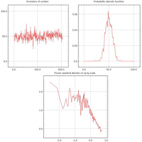
As one could expect, if herding is weak, \( \sigma_1 \approx\sigma_2 \gg h \), system state fluctuates around some intermediate value (see Fig 1.). In such case agents do not organize themselves into groups - they make individual decisions. As herding is not important in this case, intermediate value around which fluctuations occur depends on the ratio of \( \sigma_1 \) and \( \sigma_2 \).

Fig. 1:Weak herding behavior (\( h=0.02 \), \( \sigma_1 = \sigma_2 =1 \)).

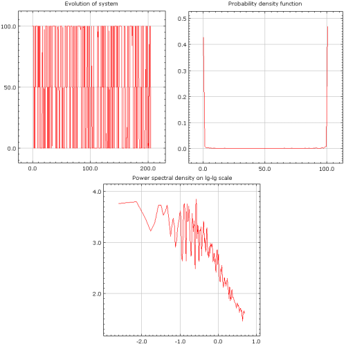
In other extreme case, \( \sigma_1 \approx \sigma_2 \ll h \), system behaves differently - most of ants at any given point of time use only one food source (see Fig. 2.). At some times switches between food sources occur. Interestingly enough weak individualism plays major role in observed dynamics as switches occur due to majority of ants choosing to follow individualists. If we turn off individualism within the system, its state will converge to stable states at \( x=0 \) or \( x=N \) - there will be no further fluctuations.

Fig. 2:Strong herding behavior (\( h=50 \), \( \sigma_1 = \sigma_2 =1 \)).

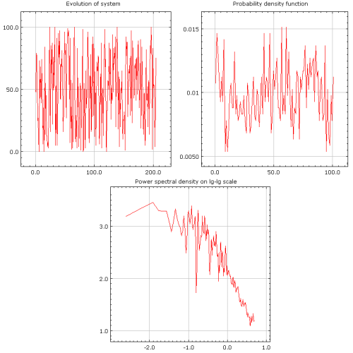
Dynamics in the extreme cases illustrate mostly single one mechanism behind the model, thus most interesting behavior can be observed in between. If two different behavior mechanics are balanced, \( h\approx \sigma_1 \approx \sigma_2 \), agents at the same time tend to form groups and act on their own accord. Interestingly in such case entropy of the system is at its or near its maximum as probabilities of observing each system state are very similar (see Fig 3.).

Fig. 3:Balanced behavior case (\( h=1 \), \( \sigma_1 = \sigma_2 =1\)).

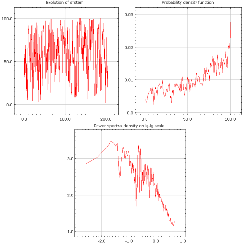
In all previous examples behavior of the system is symmetrical - neither food source is preffered, \( \sigma_1 \approx \sigma_2 \). But what happens if one of the food sources is preferred, say \( \sigma_1 > \sigma_2 \)? As one would expect in such case probability density function maxima moves a bit towards larger system state, \( x \), values. This means that first food source, the one which is exploited by \( x \) ants, becomes preferred and is used more frequently than the other one (see Fig 4.).

Fig. 4:Asimmetric behavior case (\( h=1 \), \( \sigma_1 =1.2 \), \( \sigma_2 =0.8 \)).

Applet

In the previous section of this article it was shown that \( \Delta t \) values must be limited from the above in order for model equations to have mathematically correct interpretation. In the program below we have chosen to use one of the previous inequalities to define actual value of \( \Delta t \):

\begin{equation} \Delta t = \frac{2 \kappa}{N (\sigma_1 + \sigma_2 + h N)}, \end{equation}

note that here parameter \( \kappa \) has appeared. This parameter is responsible for precision of the calculations and allows user to fulfill requirements set by the previous inequalities for \( \Delta t \) - one just need to set \( \kappa \) value to 1 or other smaller positive number. In most of the cases \( \kappa \approx1 \) will suffice.

References

• A. P. Kirman. Ants, rationality and recruitment. Quarterly Journal of Economics 108: 137-156 (1993).
• S. Alfarano, T. Lux, F. Wagner. Estimation of Agent-Based Models: The Case of an Asymmetric Herding Model. Computational Economics 26: 19-49 (2005).
• S. Alfarano, T. Lux, F. Wagner. Time variation of higher moments in a financial market with heterogeneous agents: An analytical approach. Journal of Economic Dynamics and Control 32: 101-136 (2008).