Modeling wealth distribution using kinetic exchange models

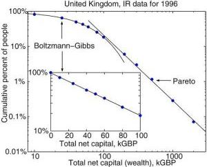
We have previously wrote about the elementary kinetic models. Now we would like to put them to a certain use - namely we would like to model wealth distributions. The problem is that the stationary distribution of the elementary kinetic models, as we have shown before, is Boltzmann-Gibbs distribution, while the empirical distribution of wealth has a power law tail (see Fig. 1). Therefore we will need some essential modifications to replicate the empirical distribution.

Fig. 1:Inverse cumulative distribution function of wealth. Data are of the United Kingdom from 1996. Figure taken from an article by Patriarca and Chakraborti (2013).

One of the keys to success in this case is the introduction of the more realistic saving mechanism. Previously we have assumed that the saving propensity is fixed - namely that all particles store the same amount of energy. Yet a more realistic assumption may be made - particles may save the energy based on the proportions! Namely the can save a certain percentage of current energy to use in the future interactions. For the sake of simplicity let us start by assuming that this saving propensity is the same for all particles and equals \( \kappa \). Now one can introduce it into the reshuffling model:

\begin{equation} \Delta w_{ij} = (1-\kappa) [ (1-\varepsilon) w_i(t) -\varepsilon w_j(t) ] . \end{equation}

One can convince himself that the stationary probability density function (abbr. PDF) of this model is given by the Gamma distribution [1]:

\begin{equation} p(w) \sim w^{n-1} \exp(- n w), \end{equation}

here \( n = 1 +\frac{3 \kappa}{1-\kappa} \). In physics similar shape of distribution is seen for the ideal gas particle energies in the \( d \)-dimensional case, where \( n \) equals half of the spatial dimension \( n=d/2 \). It should be pretty straightforward to relate the abstraction of saving propensity and the dimensionality of the system: \( \kappa = \frac{d-2}{d+4} \). The impact of the proportional saving propensity can be seen in the interactive HTML5 applet below.

Note that in this model the stationary distribution still behaves as exponential in the limit of large energies, while we want to obtain power-law behavior! Though it is note hard to modify this model to have this kind of asymptotic behavior. One just needs to assume that agents may have heterogeneous saving propensity! In such case \( \Delta w_{ij} \) is given by

\begin{equation} \Delta w_{ij} = (1-\kappa_i) (1-\varepsilon) w_i(t) -(1-\kappa_j) \varepsilon w_j(t) , \end{equation}

here \( \kappa_n \) are the saving propensities of different particles, which are uniformly distributed in the interval \( [0,1] \) (this randomization is done during model initialization). This simple assumption is enough to reproduce the power law tail! This result suggests that agent heterogeneity is a very powerful and important tool. You can see the power-law distribution (note that the plot is log-log) in the HTML5 applet below.

How did this happen? Why we have obtained power-law distribution under so simple assumptions? The answer lies in a fact that Gamma distribution is still a correct approximation of any single particle energy distribution. Yet the sum over each different particles energy distribution yields a power-law PDF. Mathematically, if \( \kappa_i \) are evenly distributed in \( [0,1] \) and the number of particles, \( N \), is sufficiently large, one can obtain that

\begin{equation} p(w) = \frac{1}{N} \sum_{i=1}^N C_i w^{\frac{3\kappa_i}{1-\kappa_i}} \exp\left[-\left(1+\frac{3\kappa_i}{1-\kappa_i}\right) w \right] \propto w^{-2} . \end{equation}

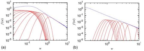
One can understand this visually by looking into the Fig. 2. Here all particles were grouped into the groups, which have similar \( \kappa \) values. As you can see, red monotonic curves, the energy distribution in each interval (except the last one, \( \kappa_i \in (0.9,1] \)) is rather well approximated by a Gamma distribution (subfigure (a)). If we would group the particles of the last interval into a smaller groups (\( (0.9,0.91] \), \( (0.91, 0.92] \), \( (0.92, 0.93] \) and etc.) we would see that each of this smaller groups once again have a distribution of energies similar to the Gamma distribution (subfigure (b)). Yet the sum over all particles has a power-law tail and is given by blue dashed curve.

Fig. 2:Sum over Gamma distributions (red curves) becomes power-law distribution (blue curve). In the subfigure (a) we can see the energy distributions of particles in certain intervals of κ values, which is approximately Gamma distributions except for the last one. While in the subfigure (b) we see that if last interval of κ values is broken up into smaller intervals, then the particles in those smaller intervals once again have Gamma-like distrubtions of their energy. Figure taken from an article by Patriarca and Chakraborti (2013).

Only small detail is left to be reproduced - empirical distribution has a "bump". This may be introduced into the model by assuming that certain fraction of particles, \( p_0 \), has a fixed saving propensity, \( \kappa_0 \), while all other particles have a random saving propensity. In such case one Gamma distribution in the sum is strongly emphasized thus forming a "bump", while the sum over others allows to obtain the power-law tail.

Therefore by playing with \( p_0 \) and \( \kappa_0 \) parameters one can reproduce the empirical wealth distribution [1]. The only drawback is that the exponent of power-law tail is fixed and set to 2.

References

• M. Patriarca, A. Chakraborti. Kinetic exchange models: From molecular physics to social science. American Journal of Physics 81: 618-623 (2013). doi: 10.1119/1.4807852.