PSD of a point process with non-exponential inter-event times
In the previous post we have seen that the Poisson process generates white noise, which is not unexpected consequence of exponential distribution being a limit of geometric distribution. So, if we use non-exponential inter-event time distribution, we introduce memory into the process. As the distribution of inter-event times is no longer exponential, we now have not a Poisson process, but a point process.
Weibull distributed inter-event times
Back in 2020 we have improved our statistical model of COVID-19 by assuming that patient recovery times are distributed according to the Weibull distribution. Weibull distribution is a generalization of the exponential distribution, which takes into account ageing effects:
\begin{equation} p(\tau) = k \lambda \left(\lambda \tau \right)^{k-1} \exp\left[ - \left(\lambda \tau \right)^k \right] . \end{equation}
If its shape parameter \( k = 1 \) there are no ageing effects (the event rate remains constant) and the distribution is equivalent to the exponential distribution. For lower \( k \) the event rate decreases with time, which means that extreme (both short and long) event times become more frequent. For higher \( k \) the event rate increases in time, thus most events happen at intermediate times.
While examining Weibull distribution in our case is a rather natural choice, its characteristic function is somewhat too complicated:
\begin{equation} \chi_\tau(f) = \sum_{n=0}^{\infty} \frac{(2 \pi i f)^n}{n! \lambda^n} \Gamma\left( 1 + \frac{n}{k} \right) . \end{equation}
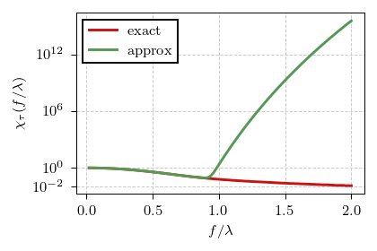
Typically one would take first few terms of the sum, but there are a couple of important caveats in this particular case. First of all the sum does not converge for \( k < 1 \), rewrite \( n! \) as \( \Gamma( 1 + n ) \) to see that it is always much smaller than \( \Gamma ( 1 + n / k ) \). Yet even with \( k > 1 \), we need far more than three terms (up to the second order term) we would typically take. In the figure below you can see the comparison between the exact result for \( k = 2 \) (red curve) and the approximation using first \( 50 \) terms (green curve).
 Fig. 1:The exact characteristic function for k=2 case (red curve) and its approximation obtained by retaining first 50 terms (green curve).
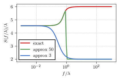
The view is quite terrible and thus results in misleading analytical approximation of the PSD (see the figure below). Well, not good. So let us keep the analysis purely numerical in this particular case.
 Fig. 2:The exact PSD obtained for the k=2 case (red curve) and the approximation obtained by retaining first 50 terms (green curve) or first 3 terms (blue curve).
As you can verify using the interactive app below, the qualitative shape obtained for the \( k = 2 \) case is reproduced with other \( k > 1 \). In \( k = 1 \) case Weibull distribution becomes identical to the exponential distribution, and thus the earlier derived result is reproduced.
The intuition
So, the question one could ask would be why the power spectral density is lower for frequencies lower than even rate, and higher for frequencies larger than event rate. I explain this result to myself by thinking that as \( k \) grows larger extremely small inter-event times become extremely unlikely. Thus there is very little "action" on the smallest time scales.
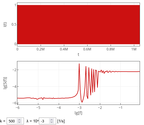
But larger \( k \) imply that extremely long inter-event times also become notably less likely. But for some reason, this can't be as quickly seen in the power spectral density. As both short and long inter-event times become less likely, inter-event times in the vicinity of \( 1 / \lambda \) becomes more likely. Thus at certain point we should start observing signs of the periodicity in the spectral density. And this is indeed true as is shown in the figure below.
 Fig. 3:Power spectral density of the point process with Weibull inter-event times for k=500.
Interactive app
Interactive app below samples time series from the point process with inter-event times being sampled from Weibull distribution. To verify the analytical intuitions above, we perform spectral analysis on the discretized time series. The discretized time series are obtained by counting the number of events inside unit time windows (the top plot). In total \( 2^{20} \) (roughly one million) such time windows are observed each time "Generate" button is pressed. PSD of the sampled series is shown in the bottom plot as a red curve.
