Three group Kirman's agent-based model for financial markets

As we have seen previously application of the original Kirman's model enables reproduction of single power law spectral density [1]. While actual financial markets and sophisticated stochastic models [2] have double power law spectral density - i.e., fractured spectral density. Thus it would be nice to obtain fracture of spectral density by improving application of Kirman's agent based model towards financial markets.

One can create more sophisticated model in various ways. The two main options are a possibility to combine multiple stochastic models obtained while analyzing stochastic treatment of Kirman's model [3] and a possibility extend agent-based model itself [4]. Speaking of latter possibility, it is possible to improve agent-based model by introducing additional agent groups or splitting old ones. Despite of previous lack of success, even multi-group agent-based models [5, 6, 7] were unable to reproduce fracture in spectral density, this option still looks promising as one does not need to make strong assumptions.

Three group financial market model

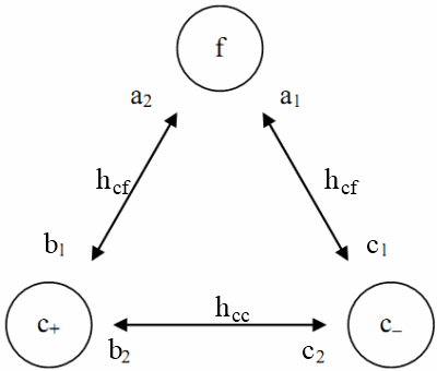
In this text we will attempt to obtain fractured spectral density without making any strong assumptions. Similar, though broader, discussion is available in [4]). In previous application we have considered dynamics only between chartist and fundamentalist groups [1], while it is natural to expect that chartist agents may disagree in their expectations and thus devide into additional groups (or subgroups) - pessimists and optimists. Therefore now all three groups (see Fig. 1) may interact among themselves.

Fig. 1:Three groups interactions: f - fundamentalists, c+ - chartists optimists, c- - chartists pessimists. Symbols written near the bubbles correspond to the parameters related to individual decision, while symbols written on the inter-connections are related to herding.

Group interactions are mathematically described in the terms of original Kirman's model, where relevant parameters somewhat differ (see Fig. 1). These now six, as we have interactions between three groups, transition equations mathematically are expressed as:

\begin{equation} p( c_{-} \rightarrow f) = n_{c-} (a_1 + h_{cf} n_f)\Delta t , \end{equation}

\begin{equation} p( c_{+} \rightarrow f) = n_{c+} (a_2 + h_{cf} n_f)\Delta t , \end{equation}

\begin{equation} p( f \rightarrow c_{+}) = n_{f} (b_1 + h_{cf} n_{c+})\Delta t , \end{equation}

\begin{equation} p( c_{-} \rightarrow c_{+}) = n_{c-} (b_2 + h_{cc}n_{c+}) \Delta t , \end{equation}

\begin{equation} p( f \rightarrow c_{-}) = n_{f} (c_1 + h_{cf} n_{c-})\Delta t , \end{equation}

\begin{equation} p( c_{+} \rightarrow c_{-}) = n_{c+} (c_2 + h_{cc}n_{c-}) \Delta t . \end{equation}

Note that the above transition probabilities describe one agent transition between varying groups. \( a_i \), \( b_i \) and \( c_i \) in these transition probabilities stand for individual behavior, while \( h_{ij} \) describe herding tendencies. Also it is important to note that only two different herding parameters are being used - one is being used for chartist-chartist process, which we will assume to be a faster one, and chartist-fundamentalist process, which was assumed to be slower process and analyzed in [1]. As we allow only one agent to change his group during \( \Delta t \), it should be accordingly short time period. \( \Delta t \) can be treated as model parameter, though constant value will hinder numerical evaluation. Therefore it is more convenient to use variable \( \Delta t \), which can be defined by requiring that the sum of the transition probabilities is one or less:

\begin{equation} \sum\limits_i p(i) = \Delta t \sum\limits_i \pi(i) =\kappa \quad \Rightarrow \quad \Delta t =\frac{\kappa}{\sum\limits_i \pi(i)} , \end{equation}

here \( p(i) = \pi(i) \Delta t \), index \( i \) denotes all possible single transition scenarios, \( \kappa \leq 1 \) may stand for numerical evaluation precision parameter.

Model might be also improved by reducing the number of model parameters. To do so we introduce dimensionless time scale \( t = h_{cf} t_s \). After its introduction one should also substitute non-dimensionless model parameters for their dimensionless counterparts: \( A_i = \frac{a_i}{h_{cf}} \), \( B_i =\frac{b_i}{h_{cf}} \), \( C_i = \frac{c_i}{h_{cf}} \) and \( H = \frac{h_{cc}}{h_{cf}} \).

Application towards financial markets

All that is left to do now is to relate previously discussed group dynamics to the financial market observables, namely price and return. We do so by utilizing original Walras law, i.e., we assume that market maker stabilizes the market after each change to the supply and demand. We have already discussed this topic on Physics of Risk (see this text). Thus from the market maker assumption, and by using previous experience, we can draw expression of price

\begin{equation} P(t) = P_f(t) \exp \left[ r_0 \frac{N_c(t)}{N_f(t)}\xi(t) \right] = P_f(t) \exp \left[ -r_0\frac{N_{c+}(t)-N_{c-}(t)}{N_f(t)} \right] , \end{equation}

and thus return, under the assumption that fundamental price remains constant,

\begin{equation} r_{T}(t)=\ln \frac{P(t)}{P(t-T)} = r_0 \left[-\frac{N_{c+}(t)-N_{c-}(t)}{N_f(t)} +\frac{N_{c+}(t-T)-N_{c-}(t-T)}{N_f(t-T)} \right] . \end{equation}

As in this text we are only interested in spectral density we can drop \( r_0 \) from the definition of return.

Model results

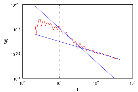
In [4] paper model's spectral density was analyzed using different parameter sets. In Fig. 2 we can see reportedly best fractured spectral density (its powers, \( \beta \), are close to empirical ones). Qualitatively similar results can be obtained with H being larger than 10 and smaller than 1000. Otherwise spectral densities of chartist-chartist and chartist-fundamentalist process do not sufficiently differ (H smaller than 10) or overlap (H larger 1000).

Fig. 2:Spectral density (red curve) of absolute return time series obtained by numerically evaluating the discussed model and its power law fits (blue curves). Powers of power law fits: \( \beta=0.68 \), \( \beta=0.22 \). Model parameters: \( a_1=a_2=b_1=c_1=30 \), \( b_2=c_2=500 \), \( h_{cf}=1 \), \( H=50 \), \( T=0.001 \).

Applet

References

• A. Kononovicius, V. Gontis. Agent based reasoning for the non-linear stochastic models of long-range memory. Physica A 391: 1309-1314 (2012). doi: 10.1016/j.physa.2011.08.061. arXiv: 1106.2685 [q-fin.ST].
• V. Gontis, J. Ruseckas, A. Kononovicius. A Non-linear Stochastic Model of Return in Financial Markets. In: Stochastic Control, ed. C. Myers. InTech, 2010. doi: 10.5772/9748.
• A. Kononovicius, V. Gontis, B. Kaulakys. Agent based reasoning of the nonlinear stochastic models. Verhandlungen DPG (VI) 46: 502. Dresden, Germany, 2011.
• P. Purlys. Kirmano sąveika tarp trijų tipų agentų finansuose. Vilniaus universitetas, Kursinis darbas, 2011.
• S. Bornholdt. Expectation bubbles in a spin model of markets: Intermittency from frustration across scales. International Journal of Modern Physics C 12: 667-674 (2001).
• T. Lux, M. Marchesi. Scaling and criticality in a stochastic multi-agent model of a financial market. Nature 397: 498-500 (1999).
• S. H. Yook, H. J. Kim, Y. Kim. Agent-based generalized spin model for financial markets on two-dimensional lattices. Journal of the Korean Physical Society 52: S150-S153 (2008).