Achieving high clustering in scale-free networks

Average shortest path (sometimes network diameter), degree distribution and clustering are the three main network characteristics. Path lengths tend to be small in random network models (average shortest path and network diameter grows as \( \ln N \) or slower). Power-law degree distribution can be obtained from the Barabasi-Albert and some other models. But clustering appears to be trickier to reproduce together with the previous two. In this text we will discuss what clustering actually is and how to obtain it in random network model.

Context of the three main random network models

Below you should see a contents of the slide featured in the presentation by A. L. Barabasi (full slides may be found here: http://barabasilab.neu.edu/courses/phys5116/). On this slide the three main network formation models (Erdos-Renyi, Watts-Strogatz and Barabasi-Albert) as well as regular network structure are being compared against the main statistical properties discussed in the previous paragraph.

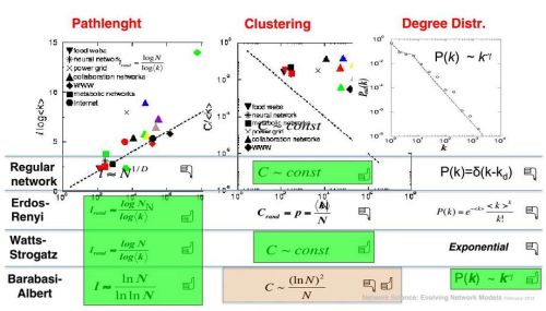
As it was already told the shortest paths are OK in all three random network models. Indeed as Watts-Strogatz model has shown - smallest amount of randomness helps to significantly decrease path lengths in networks. Degree distribution, also as it was already mentioned, seems to be OK only in case of Barabasi-Albert model (assuming that we are interested in complex networks exhibiting power-laws). While clustering is good only when regular network structures are more (purely regular network) or less (Watts-Strogatz) featured. We will use this insight later, and now let us continue with a discussion about clustering itself.

We would like to draw your attention to that on the slide degree \( k \) is used to denote node degree, while further in text we use \( d \). \( k \) is a more convenient option if the text also consider path lengths (borrowing \( d \) due to the first letter of the terms distance and diameter), but as we do not consider these properties in this text we will use \( d \) (due to the first letter of term degree).

Clustering - a measure of network density

Imagine that you have a node \( i \), which has to distinct neighbors \( m \) and \( j \). Local clustering coefficient tells us the probability that \( m \) and \( j \) are neighbors themselves. Namely if \( C_i =1 \), we would expect that all pairs of distinct \( m \) and \( j \) are connected among themselves. If on the other hand \( C_i =0 \), then there should be no edges between any pair of \( m \) and \( j \). Mathematically this can be expressed as:

\begin{equation} C_i = \frac{2 L_i}{d_i (d_i - 1)} , \end{equation}

where \( L_i \) is a number of edges between the neighbors of \( i \). Evidently \( \frac{1}{2} d_i (d_i -1) \) is a total number of pairs between the all neighbors of \( i \).

Then considering clustering of the global structure it is important to tell two distinct measures apart - global clustering coefficient, \( C \), and average clustering coefficient, \( \langle C\rangle \). The difference lies in a fact that global clustering coefficient is "weighted" by degree, while in the second case averaging is weighted by individual nodes. In some case it is very possible that these two measures will provide very contradicting results.

Further in text we will consider average clustering coefficient, but we will use a simpler notation - \( C \).

Why regular structures possess high clustering?

Fig 1.Regular network - nodes are connected as a ring, where each node has 4 edges directed to its nearest neighbors. Red color is used for the considered node and its edges. Blue circles are its neighbors and green lines are the edges between them.

The red node in the figure above has clustering coefficient of \( 0.5 \). As there is 3 edges (green lines) between its neighbors (blue circles) out of six possible pairings (\( d_i = 4 \enspace\Rightarrow \enspace \frac{4 \cdot 3}{2} = 6 \)). The number appears to be not that large, but let us consider a completely random network (Erdos-Renyi model) with the same average degree and number of nodes. It is known that clustering coefficient of the Erdos-Renyi model is equal to the edge formation probability:

\begin{equation} C_{ER} =p . \end{equation}

This probability is easily obtained from the total number of nodes and average network degree:

\begin{equation} \langle d \rangle = p N \quad \Rightarrow \quad p =\frac{\langle d \rangle}{N} . \end{equation}

In our regular network structure all nodes are the same, thus \( \langle d \rangle = 4 \). When number of nodes goes to infinity, \( N \rightarrow \infty \), the clustering coefficient of the random network with the same average degree will go to zero, \( C_{ER} \rightarrow 0 \). While clustering coefficient, \( C_{reg} \), of our regular structure will remain equal to \( 0.5 \). Regular structures are resistant to the increase in the number of nodes as at individual node level nothing changes. But can one use this insight to create scale-free model with high clustering?

A model proposed by K. Klemm and V. M. Eguiluz

In order to have high clustering we should have a lot of fully inter-connected triangles (or triads). So let us proceed as is suggested in [1]:

• Start with a full graph consisting of \( m \) nodes. Let us call these nodes "active".
• Now add a single new node and connect it to all "active" nodes.
• Add the new node to the group of "active" nodes.
• Remove one node from the group of "active" nodes. Let the probability of deactivation be inversely proportional to node degree: \( p_d(d_i) \propto \frac{1}{m+d_i} \).
• Repeat second-forth steps until you reach desired network size.

Fig 2.Scale-free network with constant clustering.

As you can see in the figure above the generated network is scale-free (the degree distribution is power-law). Yet unlike in Barabasi-Albert model the clustering coefficient remains almost constant with increasing number of nodes \( N \). Try the interactive HTML5 applet below.

Note that in this applet we have disabled automatic zoom on the graph (manually this can be done using mouse wheel). This was done in order to conserve computational power of your computer. Due to the same reasons the figure in applet are updated only after 10 steps.

References

• K. Klemm, V. M. Eguiluz. Highly clustered scale-free networks. Physical Review E 65: 036123 (2002). doi: 10.1103/PhysRevE.65.036123.