Football data analysis and modeling showcase

This year I got to teach a numerical methods course to first year students in Faculty of Physics (Vilnius University). As theory is somewhat boring and feels somewhat detached from practice, I have decided to provide students with practical showcase on how to work with empirical data. For this showcase I have selected a small subset of a larger football data set. Namely, I decided to take a look at English Premier League's 2000/2001 season.

This showcase took two lectures and a bit of time after the lectures to cleanup the code. The first lecture was mostly dedicated to empirical analysis of the data set, while the second lecture's focus was building a statistical model based on the analysis.

Empirical analysis

What was the highest scoring games during the analyzed season? We have asked this question out of simple curiosity as well as to check whether our understanding of the data is good enough to do more complex analysis. Our findings were identical to the ones reported in official statistics, so we can assume that everything works fine to this point.

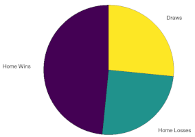
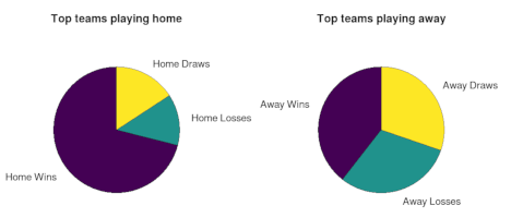
Is there evidence for a home advantage? This rather interesting question as beliefs about home advantage are as common as beliefs about "hot hands" we have written about earlier. Interestingly unlike for the "hot hands" we clearly see that home teams gain noticeable advantage against their opponents.

Fig 1.Proprotions of the games won, drawn and lost by the home teams during the English Premier League 2000/2001 season.

Fig 2.Proprotions of the games won, drawn and lost by the top 5 teams of the English Premier League 2000/2001 season playing home and away.

Is there a difference between number of goals scored home and away? This question is mostly related to the previous one. Here we see that usually teams scored more goals home than away, though there are few exceptions. All of the major exceptions were stuck in the bottom of table during the season. So I guess if you are terrible, then you are equally terrible at home and away.

------ Home / Away Goals ------
          Arsenal 45 18 2.500
      Aston Villa 27 19 1.421
    Bradford City 20 10 2.000
Charlton Athletic 31 19 1.632
          Chelsea 44 24 1.833
    Coventry City 14 22 0.636
     Derby County 23 14 1.643
          Everton 29 16 1.812
     Ipswich Town 31 26 1.192
     Leeds United 36 28 1.286
   Leicester City 28 11 2.545
        Liverpool 40 31 1.290
  Manchester City 20 21 0.952
Manchester United 49 30 1.633
    Middlesbrough 18 26 0.692
 Newcastle United 26 18 1.444
      Southampton 27 13 2.077
       Sunderland 24 22 1.091
Tottenham Hotspur 31 16 1.938
  West Ham United 24 21 1.143

Is there a difference between teams performance in the first half of a season and the second half of a season? Obviously there can be changes in team form on this time scale. These might be related to squad or managerial changes. Also there could some variance of purely statistical nature. While we have found some noticeable differences we can't make any conclusions without deeper knowledge of transfers and injuries throughout the season.

--- First / Second Half of the season ---
          Arsenal 30 33 0.909
      Aston Villa 23 23 1.000
    Bradford City 13 17 0.765
Charlton Athletic 26 24 1.083
          Chelsea 35 33 1.061
    Coventry City 17 19 0.895
     Derby County 23 14 1.643
          Everton 20 25 0.800
     Ipswich Town 27 30 0.900
     Leeds United 26 38 0.684
   Leicester City 22 17 1.294
        Liverpool 37 34 1.088
  Manchester City 25 16 1.562
Manchester United 46 33 1.394
    Middlesbrough 20 24 0.833
 Newcastle United 20 24 0.833
      Southampton 24 16 1.500
       Sunderland 19 27 0.704
Tottenham Hotspur 26 21 1.238
  West Ham United 25 20 1.250

Statistical model

Statistical model we have built based on the observations is quite similar to the one discussed by prof. Tony Padilla in the Numberphile video we have linked below. You can watch the idea to get a general idea, or review our formulas further below the video.

So initially we take a look at the league as whole. Namely we figure out baseline goal scoring capacities for all teams in the Premier League. As we know that goal scoring capacities are different for home and away teams, we calculate them separately:

\begin{equation} \langle \lambda_{HG} \rangle = \frac{\Sigma_{HG}}{380} , \qquad \langle \lambda_{AG} \rangle = \frac{\Sigma_{AG}}{380} . \end{equation}

In the above \( \lambda_{HG} \) is the home team goal scoring capacity, which is calculated by dividing total goals scored by the home teams by the number of games. Away team goal scoring capacity, \( \lambda_{AG} \), is calculated in similar manner.

Then we treat teams separately by considering their relative attacking and defensive potentials both home and away. So all in all we get four distinct numbers for each of the team. These are obtained once again by dividing goals (scored and conceded by the team home and away, divided by the number of games). So team attack and defense potentials, if the team plays home, is given by:

\begin{equation} \mathrm{Att}_{H,i} = \frac{1}{\langle \lambda_{HG} \rangle} \cdot \frac{\Sigma_{HG,i}}{19} , \qquad \mathrm{Def}_{H,i} = \frac{1}{\langle \lambda_{AG} \rangle} \cdot \frac{\Sigma_{AG,-i}}{19} , \end{equation}

and if the team plays away:

\begin{equation} \mathrm{Att}_{A,i} = \frac{1}{\langle \lambda_{AG} \rangle} \cdot \frac{\Sigma_{AG,i}}{19} , \qquad \mathrm{Def}_{A,i} = \frac{1}{\langle \lambda_{HG} \rangle} \cdot \frac{\Sigma_{HG,-i}}{19} . \end{equation}

In the above \( \Sigma_{HG,i} \) and \( \Sigma_{AG,i} \) are the total number of home and away goals for team \( i \), while \( \Sigma_{HG,-i} \) and \( \Sigma_{AG,-i} \) are the total number of home and away goals against team \( i \).

So when we generate a single game we can simply sample from Poisson distribution to get total number of goals scored by home team, lets say \( i \), and away team, lets say \( j \):

\begin{equation} g_{h,i} \sim \mathrm{Poiss}(\langle \lambda_{HG} \rangle \cdot \mathrm{Att}_{H,i} \cdot \mathrm{Def}_{A,j}) , \end{equation}

\begin{equation} g_{a,j} \sim \mathrm{Poiss}(\langle \lambda_{AG} \rangle \cdot \mathrm{Att}_{A,j} \cdot \mathrm{Def}_{H,i}) . \end{equation}

You might be wondering why we use Poisson distribution. We do so because we assume that goal scoring is a random process (similar to radioactive decay and such). Namely we assume that time between goals is exponential distributed. This assumption appears to be rather fake, but this is indeed true for the empirical data [1]. Though we can't see this directly in the considered data set, alternatively we could check directly the distribution of goals in a game, but this thought came rather late and we haven't done this during the lecture as we were running out of time.

Matlab's scripts

I have made the Matlab (actually developed in GNU Octave, but the code should be compatible with Matlab) code available on GitHub: https://github.com/akononovicius/football-model.

References

• M. Levene, A. Kononovicius. Empirical Survival Jensen-Shannon Divergence as a Goodness-of-Fit Measure for Maximum Likelihood Estimation and Curve Fitting. arXiv:1809.11052 [stat.ME].