Peter principle

Last time I have shared a video about the Peter principle, which states that "in a hierarchy, every employee tends to rise to their level of incompetence." Actually, I have heard about this principle before in the scientific context. Prior to the video, I have heard about this principle from a group of Italian physicists, economists and mathematicians had working on a research project about benefits of random strategies [1]. On of their works was about the Peter principle. So, lets explore!

Model

First we need to be the hierarchy. Let us build a simple hierarchical tree network. This we start with the top node, which corresponds to CEO or owner. That node is connected to three branches (their juniors). In turn, each of the junior nodes have their own three juniors (three branches). Formation of hierarchical relationships (or branching of the network) repeats until the bottom level. The "bottom" nodes are low-rank recruits who do not have any juniors. In the app below we have six hierarchical levels including the CEO.

Our choice of the branching factor (how many branches stem from the top parent nodes) and the number of generations (how many levels there are) is purely arbitrary. These choices shouldn't have any qualitative impact on the results. While we make some arbitrary choices here, we still follow the general logic outlined in [1].

To make the simulated workplace realistic, each worker (node) should have competence and age attributes. Competence is clearly important for our purposes, while age provides an additional mechanism influencing when workers leave. Specifically, workers will leave the simulated workplace either upon retirement or if they become incompetent.

Worker retirement and layoffs

When a worker leaves the simulated workplace, they will be immediately replaced by one of their juniors. If the worker is of the lowest rank, they will be replace by a random generated worker. Random worker will start with a random age between \( 18 \) and \( 25 \) (uniformly distributed), and a random competence score between \( 0 \) and \( 1 \) (uniformly distributed). When replacing their supervisor, the node will change their competence score according to the following formula,

\begin{equation} C(t+1) = \rho \cdot C(t) + ( 1 - \rho ) \cdot \xi . \end{equation}

In the above \( \xi \) stands for the uniform random variate, while \( \rho \) is the model parameter having the meaning of competence correlation. If the competence of the worker falls below a threshold value (we have set it to \( 0.1 \) in the app below), then they will be laid off during the next simulation step. As soon as worker gets laid off, new wave of promotions is triggered.

While the competence changes only on promotion, the age gets incremented during each simulation step. If the worker reaches retirement age (arbitrarily set to \( 65 \) in the app below), they will immediately retire. Once they retire, they will trigger promotions.

Promotion algorithms

The model is not fully defined without a promotion algorithm. Without it we wouldn't know whom of the three juniors to promote. The app below implements four different approaches.

• Pick best. Junior with greatest competence is selected.
• Pick worst. Junior with lowest competence is selected.
• Random pick. Random junior is selected.
• Pick best or worst. There is an equal change that best or worst junior will be selected.

Calculating company efficiency

After all layoffs, retirements and promotions have been dealt with, company efficiency is calculated. First of all, competence across each level is being averaged. Then weighted average across the levels is calculated. Mathematically company efficiency is defined as

\begin{equation} E = \sum_{i=0}^{L-1} \left( \frac{w_i}{N_i} \sum_{j=0}^{N_i-1} C^{(i,j)} \right) . \end{equation}

In the above \( L \) is the number of levels in the organization, \( w_i \) is the weight (relative importance) of the \( i \)-th level, \( N_i \) is the number workers at the \( i \)-th level, \( C^{(i,j)} \) is the current competence of \( j \)-th worker on the \( i \)-th level. Note that with this notation zero-th level corresponds to the CEO, while \( L-1 \)-st level contains workers of the lowest rank.

In the app below we have \( L = 6 \) and \( N_i = 3^i \). We calculate the importance of each hierarchical level as follows,

\begin{equation} w_i = (1 + \Delta w)^{L-i-1} = (1 + \Delta w)^{5-i} . \end{equation}

Here, \( \Delta w \) is a parameter that controls how the importance of hierarchical level changes with rank. A positive value means higher-ranking workers are given more weight, while a negative value means their importance decreases. The app allows you to choose \( \Delta w \in {-0.8, -0.5, -0.25, 0, 0.25, 0.5, 1.0} \). Notably, choosing an extreme \( \Delta w \) value, may have a qualitative impact on the results as choosing \( \Delta w < \frac{B-1}{B} \) (where \( B \) is the branching factor) makes higher rank worker contribute less than a \( B \) lower rank workers.

Results

When competence is transferred between the ranks

The results when common sense hypothesis (as defined in [1]; we refer to this hypothesis as "Transfer" hypothesis) holds, are trivial. "Pick best" promotion strategy produces the best efficiency, while "Pick worst" produces the worst outcomes.

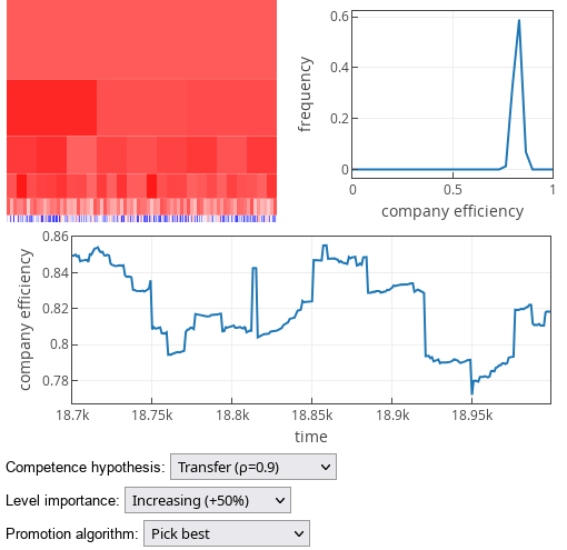Fig. 1:'Pick best' promotion strategy results under competence transfer hypothesis.

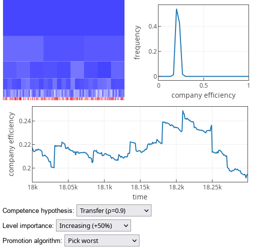Fig. 2:'Pick worst' promotion strategy results under competence transfer hypothesis.

On the other hand "Pick random" promotion strategy produces company efficiencies spread around the mean random competence, \( E \approx \langle C \rangle = 0.55 \).

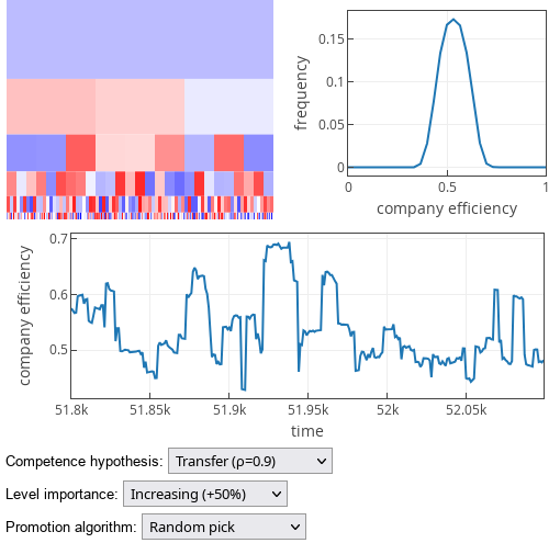Fig. 3:'Random pick' promotion strategy results under competence transfer hypothesis.

"Pick best or worst" promotion strategy produces bimodal distribution centered around the mean random competence, \( \langle C \rangle = 0.55 \).

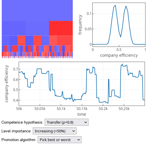Fig. 4:'Pick best or worst' promotion strategy results under competence transfer hypothesis.

When competence required for each rank is uncorrelated

The results when the Peter principle hypothesis (as defined in [1]; we refer to this hypothesis as "Randomization" hypothesis) holds, are less trivial. In this case, "Pick worst" promotion strategy yields the best company efficiency.

Though the result is unexpected only at the first glance. Namely, "Randomization" hypothesis implies that competences required at each hierarchical level are unrelated. "Promotion" in this case means that a worker gets another opportunity to find something they are good at. When we "promote" the worst worker, we effectively remove bad competence score from the pool and draw completely new competence score, which is likely to be better, because we compare the new sampled value with a bad value.

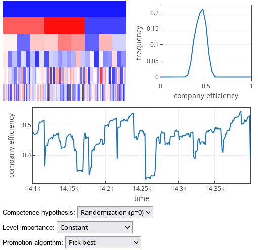Fig. 5:'Pick best' promotion strategy results under competence randomization hypothesis.

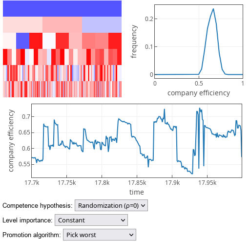Fig. 6:'Pick worst' promotion strategy results under competence randomization hypothesis.

Note that the size of the effect depends on how the level of importance scales with increasing rank. We have chosen to show this effect when the importance of each rank is identical, i.e., \( \Delta w = 0 \).

In practice promoting the worst workers would feel unnatural. So, the solution suggested by the authors [1] was to promote randomly! As only a random strategy performs consistently well whether the "Randomization" hypothesis or the "Transfer" hypothesis holds. This observation has won the authors the Ig Nobel Management Prize in 2010.

What I have found interesting

In research it is a commonly said that most work is being done by doctoral students and postdocs, while principal investigators (tenured professors) live off their students. This observation implies that the level of importance of each rank could decrease. What happens then? Well, promoting the best still seems to make sense!

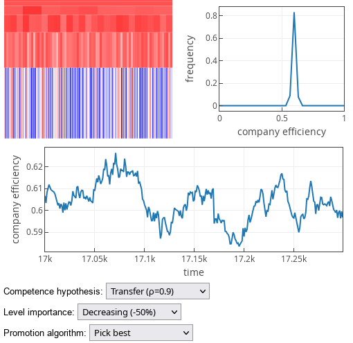Fig. 7:'Pick best' promotion strategy when lower ranks have greater importance.

This is likely the result of the fact that the lowest rank consists of a large number of random individuals. While, the worst of them remain at the lowest rank through out their worklife, a lot of them are constantly being replace by new randomly generated recruits. Thus their average competence will not be far of the average random competence, \( \langle C \rangle = 0.55 \).

Note that the figure above was obtained with \( \Delta w = -0.5 \). If we set \( \Delta w = -0.8 \) instead, then "Pick best" will no longer produce the better outcome. This is because with \( \Delta w = -0.8 \) (which notably less than \( \frac{2}{3} \)) most total work is actually done by the lowest ranked workers (each higher level does less and less of the total work).

Interactive app

Lots of things were already covered in the text above. So you can just jump straight into the app to explore the simulated workplace. Though, there is still one thing that remains to be explained. It is the upper left plot. This plot shows the hierarchical structure of the simulated workplace and how the competence is spread out across the ranks. Each individual agent (rectangular block) is colored based on their competence attribute. They are colored blue (cold) if their competence is low, and red (hot) if it is high. The width of each block depends on the number of coworkers of that hierarchical rank, while the height of each block indicates the relative importance of each hierarchical rank.

Note that, if you change any of the model parameters and press "Continue" button, then the model parameters will be reset to their values used in the simulation. To change the model parameter values you will need to press "Start" button and start the new simulation.

References

• A. E. Biondo, A. Pluchino, A. Rapisarda. The Beneficial Role of Random Strategies in Social and Financial Systems. Journal of Statistical Physics 151: 607-622 (2013). doi: 10.1007/s10955-013-0691-2. arXiv:1209.5881 [physics.soc-ph].