Power-law distribution from superposition of exponential distributions

In the previous post we have asked a simple question - what if gap duration is distributed according to a power-law distribution. Our answer was an apparently pure 1/f noise. But how could the power-law distribution arise? While in some materials some quantities indeed follow power-law distribution (such as blinking times in quantum dot experiments [1]), most materials have exponentially distributed generation and/or recombination times. So then, can we construct a power-law distribution from superposition of exponential distributions?

Indeed we can. From purely mathematical perspective let us sample from an exponential distribution. Let the rate of that distribution be distributed according to a power-law distribution,

\begin{equation} p(\lambda) \propto \frac{1}{\lambda^\alpha} . \end{equation}

To make normalization of this distribution possible for any \( \alpha \) let us assume that \( \lambda \) is confined to \( [ \lambda_\text{min}, \lambda_\text{max} ] \) interval. Then the sampled values \( x \) will follow a power-law distribution. Probability density function of this distribution is

\begin{align} p(x) & \propto \int_{\lambda_\text{min}}^{\lambda_\text{max}} \lambda^{1-\alpha} \exp(-\lambda x) \mathrm{d} \lambda = \nonumber \\ & = [\Gamma(2-\alpha, \lambda_\text{min} x) - \Gamma(2-\alpha, \lambda_\text{max} x) ] \cdot x^{-2+\alpha} . \end{align}

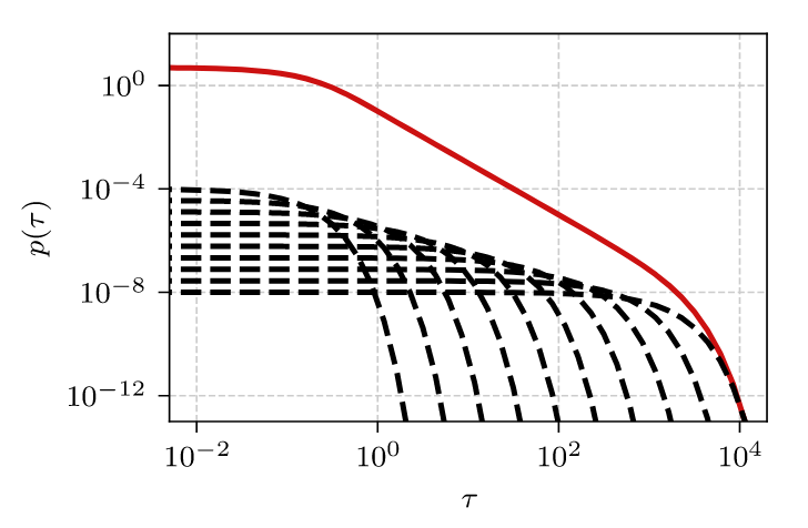
Visual intuition of what is happening is encompassed in a figure from our recent work [2], which we also reproduce here (see Fig. 1). In Fig. 1 we have shown \( \alpha = 0 \) case, which results in the inverse square law. Note that the dashed black curves visually form a simple inverse law, which when integrated becomes the inverse square law.

Fig. 1:How the integration over exponents (black dashed curves) results in a power-law distribution (red curve). Only few selected exponents shown for visualization purpose. α=0 case is shown.

Let \( \frac{1}{\lambda_\text{max}} \ll x \ll \frac{1}{\lambda_\text{min}} \), then:

\begin{equation} p(x) \approx \frac{(1-\alpha) \Gamma(2-\alpha)}{\lambda_\text{max}^{1-\alpha} - \lambda_\text{min}^{1-\alpha}} x^{-2+\alpha} . \end{equation}

The above works almost all \( \alpha \) (the only exception are positive integer values). For closest \( \alpha = 1 \) case we can show that:

\begin{equation} p(x) \approx \frac{1}{\ln\left(\lambda_\text{max}\right) - \ln\left(\lambda_\text{min}\right)} x^{-1} . \end{equation}

The other cases are less interesting to us, because they lead either to the uniform distribution, or to the strange ("unnatural" might be a better word for it) distributions with increasing \( p(x) \). Furthermore, having in mind the earlier post, we mostly care about \( \alpha = 0 \) case, which leads to \( p(x) \sim 1/x^2 \), and its vicinity.

How this is related to the random telegraph noise? Well, it allows us to avoid assuming power-law distributions to obtain 1/f noise. All we need is just uniformity of detachment rates [2]. Replacing the power-law distribution in this way has few mathematical consequences (the results from [3] still hold), but lead to a couple new insights into the low-frequency cutoff problem [2], some of these we will probably discuss some time in the future.

Interactive app

The app below allows you to see how the probability density functions of rates, \( \lambda \), and "final" sample values, \( x \), change when you tweak the parameter values. It is important to note that the \( p(\lambda) \) plot (top one) has double linear axes, while \( p(x) \) plot (bottom one) has double logarithmic axes. We made this choice, because for us most interesting case is when \( \alpha = 0 \) and \( \lambda \) follows a uniform distribution, which looks best when presented on double linear axes. As usual we show the simulation result by a red curve, and theoretical fit (bottom figure only) by a dark gray curve.

Given enough time, the app will reproduce probability density function with a power-law slope for the intermediate values. While for the extreme values, exponential cutoffs should be visible. Cutoffs appear quicker for positive \( \alpha \).

References

• P. Frantsuzov, M. Kuno, B. Jankó, R. A. Marcus. Universal emission intermittency in quantum dots, nanorods and nanowires. Nature Physics 4: 519–522 (2008). doi: 10.1038/nphys1001.
• A. Kononovicius, B. Kaulakys. 1/f noise in semiconductors arising from the heterogeneous detrapping process of individual charge carriers. Journal of Statistical Mechanics 2024: 113201 (2024). doi: 10.1088/1742-5468/ad890b. arXiv:2306.07009 [math.PR].
• A. Kononovicius, B. Kaulakys. 1/f noise from the sequence of nonoverlapping rectangular pulses. Physical Review E 107: 034117 (2023). doi: 10.1103/PhysRevE.107.034117. arXiv:2210.11792 [cond-mat.stat-mech].