Power-law distribution from superposition of normal distributions

Last time we have seen that we can recover power-law distribution from a superposition of exponential distributions. This idea served a basis for our [1] paper. When presenting some of these results at a conference I was asked question if exponential distribution is necessary, can't one use normal distribution instead?

The answer to the question I have been posed is yes. Though I wasn't able to answer it at the time. During conferences my brain switch to "general idea" mode, and often misses even most trivial technical details.

Implementing superposition of normal distributions

So, we can use the normal distribution, but we need to discuss how to do it. First recall that our purpose is to generate power-law inter-event time distribution. By definition, power-law inter-event times must be positive. Thus we need to truncate the normal distribution to positive values. Let us implement this restriction as follows: if negative value is generated, it is discarded and a new value is sampled from a normal distribution with the same parameter values.

The second thing we need to discuss is how the parameter randomization is applied. Notably, the normal distribution is described by two parameters, mean \( \mu \) and standard deviation \( \sigma \), and not one (as was the case with exponential distribution). Thus we can choose to randomize either of them or even both of them. The app below allows you to make this choice.

In the spirit of the previous post we still assume that parameter values are sampled from a bounded power-law distribution:

\begin{equation} p(\theta_i) \propto \frac{1}{\theta_i^{\alpha_i}} . \end{equation}

In the above the index \( i \) helps us differentiate between the distributions for mean and standard deviation parameters of the normal distribution.

Thus to generate observable \( x \), we first sample \( \mu \) and \( \sigma \) from the bounded power-law distributions. Parameters of these distributions are predetermined (they are input parameters, if I may call them that). When a new pair of \( \mu \) and \( \sigma \) are obtained, then \( x \) is sampled from the normal distribution with respective parameter values \( \mathcal{N}\left(\mu, \sigma\right) \).

Distribution of \( x \)

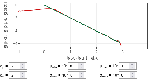
If \( \alpha_\mu = \alpha \) and \( \alpha_\sigma = \alpha \), then the probability density function of \( x \) will exhibit power-law scaling behavior, \( p(x) \sim x^{-\alpha} \). If the value of either \( \mu \) or \( \sigma \) is fixed, then the scaling exponent will be determined only by \( \alpha_i \) of the remaining randomized parameter.

Fig 1.Sample case for when the standard deviation is fixed. Red curve shows p(x), green curve - p(μ), blue curve - p(σ).

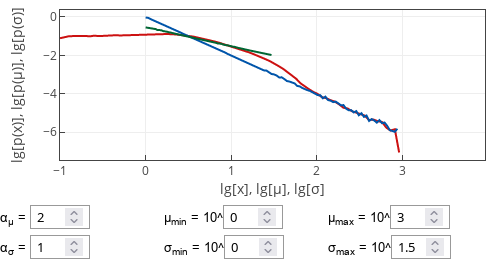
If both parameters are randomized and the corresponding exponents are different, then \( x \) distribution will often exhibit double power-law scaling behavior. Namely, there will be two ranges of values, one with \( p(x) \sim x^{-\alpha_\mu} \) and the other with \( p(x) \sim x^{-\alpha_\sigma} \).

Fig 2.Sample case for when the exponent are different. Red curve shows p(x), green curve - p(μ), blue curve - p(σ).

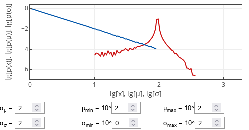
These insights are mostly for reasonable parameter values. There are some edge cases, which will have a different behavior. For example, if \( \sigma \) is fixed and larger than \( \mu_\text{max} \), then the distribution of \( x \) will become similar to normal distribution - no power-law scaling will be observed.

Fig 3.Sample case for when the mean is fixed and large (larger than maximum bound for standard deviation). Red curve shows p(x), green curve - p(μ), blue curve - p(σ).

Interactive app

This app implements sampling from normal distribution with randomized parameters. Both mean and standard deviation are sampled from a bounded power-law distribution. These parameter values are restricted to reasonable ranges, but otherwise can be freely set. Feel free to experiment with the parameter values to uncover the properties of \( x \) distribution.

Note that this app plots three probability density functions on double logarithmic axes. This is done because the most interesting behavior is observed when all distributions have power-law scaling behavior. The red curve in the plots corresponds to \( p(x) \), the green curve corresponds to \( p(\mu) \) and the blue curve corresponds to \( p(\sigma) \). Red curve is always shown, while the other curves may be hidden with respective parameter value is fixed.

References

• A. Kononovicius, B. Kaulakys. 1/f noise from the trapping-detrapping process of individual charge carriers. arXiv:2306.07009 [math.PR].

References

- A. Kononovicius, B. Kaulakys. 1/f noise in semiconductors arising from the heterogeneous detrapping process of individual charge carriers. Journal of Statistical Mechanics 2024: 113201 (2024). doi: 10.1088/1742-5468/ad890b. arXiv:2306.07009 [math.PR].