Scale-free behavior as a result of "luck and reason"

Previously we have already discussed how scale-free network could form in social systems. We have used the fact that people tend to meet new people through their friends, thus edge redirection models are perfect example of a simple social network formation model. But scale-free networks are observed in very diverse systems, thus it is highly probable that many different mechanisms for scale-free network generation may exist [1, 2]. In this text we will discuss how intrinsic random nature and tendency to optimize causes scale-free topologies to emerge in computer networks - how and why "luck and reason" may be behind the observed complexity [2].

When adding a new node (e.g., router) to the network we have to take to important factors into consideration - the cost of cable necessary to connect to certain node, \( \delta r_{ij} \) (here \( \delta \) is "cable" price per length unit and \( r_{ij} \) is the distance between the nodes), and the "fitness" of that node, \( h_j \). The most evident measure of fitness in case of computer networks is the network distance from the central node (the one which connects to other networks). The smaller the network distance is the better it is, because smaller network distance means less unnecessary load on the other parts of the network. Less load on the network means that we can use cheaper routers.

To keep thins simple we will place central node in the center of our figures, but it also may be placed randomly. Next we add network nodes one by one and place them randomly. After the placement of the node one edge is added. The edge will connect one new node to one old node. The old node, \( j \), is selected by minimizing cost:

\begin{equation} C_i = \min\nolimits_j \left\{ \delta r_{ij} + h_j \right\} . \end{equation}

In this text we will determine presence of the scale-free topology indirectly - through the probability density function of node degrees (it should at least have a power law tail) and also we will verify if preferential attachment is present in the network evolution. Estimation of the probability density function should be trivial, but the second method is more interesting. The importance of preferential attachment in the real-life growing networks can be determined by examining the rate at which nodes with distinct degrees gain new edges (increase their degree). Namely one should take network snapshots at two distinct time moments, \( \Delta t=t-t' \), and determine the change in degree, \( \Delta d_i \), for each and every node. Now the average rate can be easily determined:

\begin{equation} \Pi(d) = \left\langle \frac{\Delta d_i}{\Delta t}\right\rangle_{d_i(t')=d} . \end{equation}

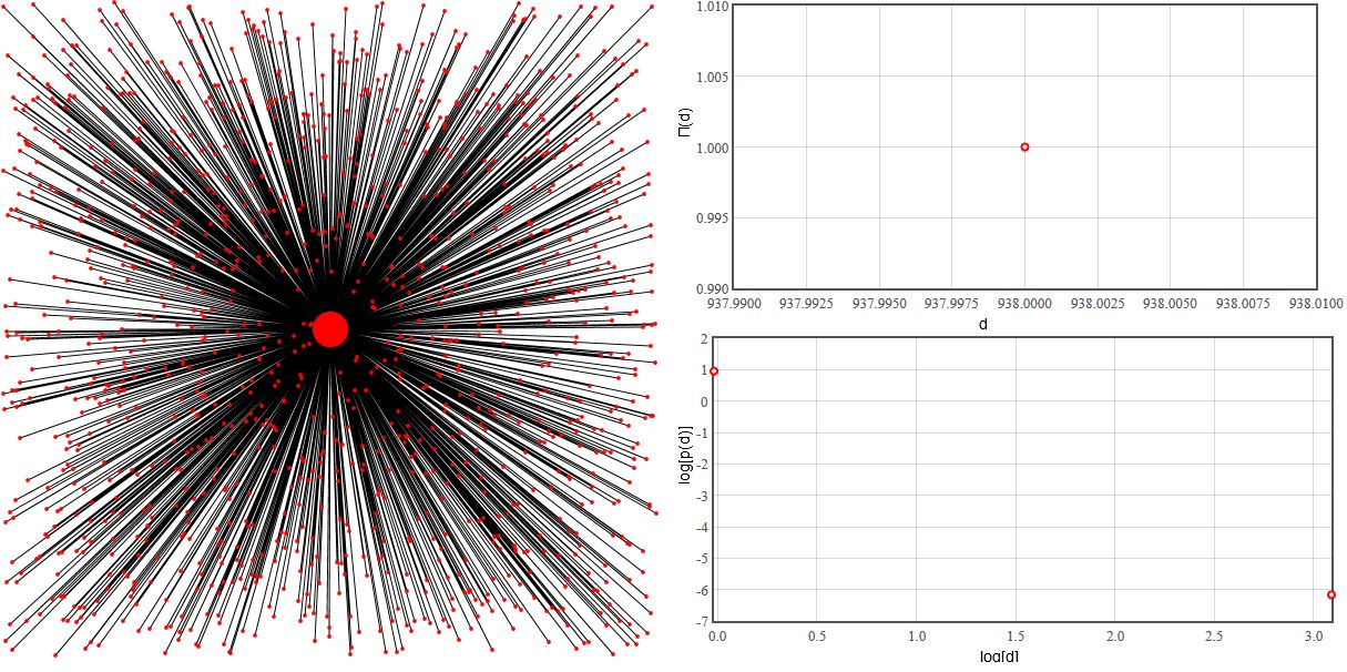
In this model \( \Pi(d) \) is a very useful indicator, which helps to single out three different network topologies generated by the model. If \( \delta \) is small (in our applet \( \delta \leq 1 \)), then network topology is hub and spoke (\( \Pi(d) \) usually has only one non-zero value). If the cable is cheap, then evidently all new nodes connect directly to the central node.

Fig 1.Small δ (δ=1). Network topology is hub and spoke - most edges are gained by central node.

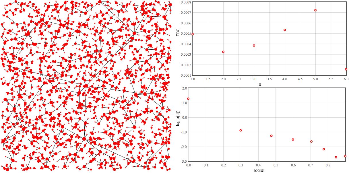
On the other hand if cable is very pricey, \( \delta \) is huge (in our applet \( \delta \gg 10 \)), then evidently all new nodes will pick only their nearest neighbor. As the new node placement is completely random, the neighbor selection also becomes random and thus our \( \Pi(d) \) becomes flat.

Fig 2.Large δ (δ=10000). Geometric distance becomes the most important factor in edge formation.

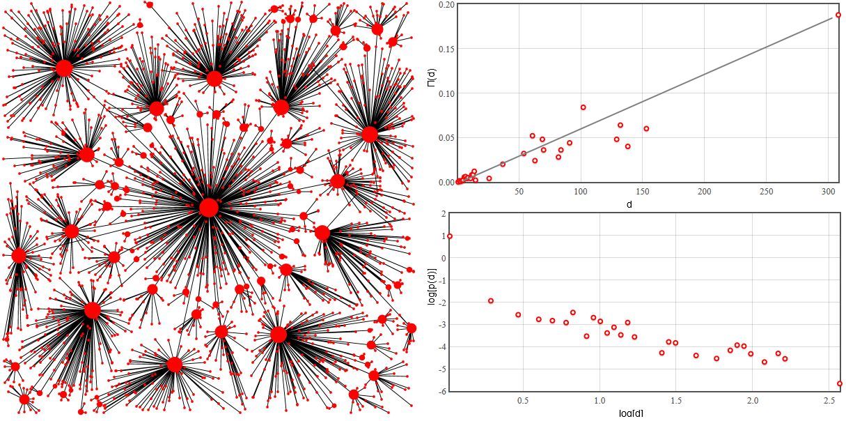
The most interesting case is obtained with intermediate prices of the cable. Namely when the influence of \( \delta \) and \( h_j \) become comparable (in our applet \( \delta \approx 5 \)). In this case both geometric and network distances are almost equally important. In this case \( Pi \) grows linearly with \( d \) suggesting that preferential attachment is present in the network formation. The probability density function of node degree's is power law thus we can draw comparisons with Barabasi-Albert model and think of the router network as scale-free network.

Fig 3.Intermediate value of δ (δ=5). Geometric and network distances are equally important.

We invite readers to test this model using HTML5 applet below.

We would like to note that during the initial steps it rather problematic to determine \( \Pi(d) \) precisely. Thus during the initial 500 steps the applet will show only approximate relationships (in the figures they will be plotted using blue dots). After the initial steps precise estimation becomes possible and the color of dots will be switched to red.

References

• R. Albert, A. L. Barabasi. Statistical mechanics of complex networks. Reviews of Modern Physics 74: 47-97 (2002). doi: 10.1103/RevModPhys.74.47. arXiv: cond-mat/0106096 [cond-mat.stat-mech].
• A. L. Barabasi. Network Science. Cambridge University Press, 2016.