Statistical physics of dating apps?

Previous summer I have stumbled upon an interesting manuscript [1], which explores dating app dynamics (?) from the perspective of statistical physics. I am not sure about the "dynamics" part, as to me it appears to be more "static" than "dynamic", but nevertheless the manuscript caught my attention and I would like to discuss some related questions in the next few posts.

In this post we will take a look at static interpretation of the "biased decisions" model from the manuscript [1].

Biased decision model

Here we will assume that there are \( 100 \) users. Each of the users will interact with every other user and either like them, or not. Probability of liking another user is given by:

\begin{equation} P(i, j) = \min \left(1, \exp\left[-\beta \delta_{ij} \right] \right). \end{equation}

In the above \( \delta_{ij} \) is the difference in attractiveness between the users. In the app below you may choose to use absolute or raw value of the difference. If absolute value is used,

\begin{equation} \delta_{ij} = \left| x_j - x_i \right|, \end{equation}

then the users will like users of similar attractiveness as themselves. If raw value is used,

\begin{equation} \delta_{ij} = x_j - x_i , \end{equation}

then users will also like everyone who is more attractive than themselves.

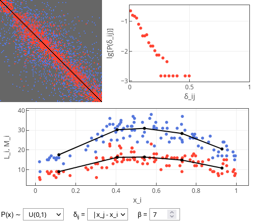
Fig. 1:When absolute difference value is used, then most likes are given to similar users

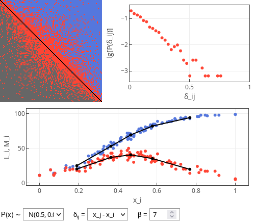
Fig. 2:When raw difference value is used, then likes are also received by the more attractive users.

In the raw difference case, the more attractive user is the more likes the user will receive. But this doesn't mean that the user will receive more matches! They will, in fact, receive less matches as they will rarely return the likes.

In the difference formulas \( x_i \) stands for attractiveness of user \( i \). This attractiveness is sampled prior to simulation from a selected distribution. The interactive app below allows you to choose from uniform distribution and truncated normal distribution. This choice doesn't significantly impact the main result - attractive users getting less matches than average ones.

Interactive app

In the interactive app below you can see three plots. The top left plot is the "relationship" matrix between the users. Its each row corresponds to user giving reaction and each column corresponds to user receiving reaction. Blue color corresponds to one-sided like (receiving user hasn't returned the like), red color corresponds to "match" (two-sided like) and dark grey indicates absence of a like. Note that the users in this plot are sorted from the least attractive (top rows) to the most attractive (bottom rows).

The top right plot shows the distribution of absolute difference in attractiveness of matched individuals (absolute \( \delta_{ij} \)). Note that y-axis is base 10 logarithm of the probability. Hence straight line, which we often see, indicates exponential distribution. Slope of the line changes with the model parameters.

The bottom plot shows number of likes (\( L_i \); blue dots) and matches (\( M_i \); red dots) received by the user of \( x_i \) attractiveness. Note that most often, the most attractive and the least attractive users receive least matches. Black lines show average values in five attractiveness bins (they are effectively a smoothening of the simulation result).

Note that this model is static - users interact among each other only once per click on "Simulate" button. As usual, feel free to explore!

References

• F. Olmeda. Towards a statistical physics of dating apps. arXiv:2107.14076 [physics.soc-ph].