Dynamical model of dating apps

In this post I continue my exploration of the [1]. Yet here I will slowly start moving away from the course of the original manuscript.

The original manuscript [1] also explores unbiased decision model. In the unbiased model users make decision only based on the attractiveness of the recipient. For some reason I do not feel that unbiased decisions are realistic (though only the data can tell this) and thus I will not explore the unbiased model.

The original manuscript is also concerned with another important feature of the dating apps: visibility of the users. It is not likely, but still somewhat possible, that I will also follow in this direction.

Still this post is within the scope of the original manuscript, as when reading it I wasn't able to understand whether static or dynamic model is considered. So here I present you a dynamic biased decision model.

Dynamic model

The dynamic model follows the premise of the static model. The only difference that users may place any number of likes and dislikes on the other users. Their decision is still based on the biased decision probability:

\begin{equation} P(i, j) = \min \left(1, \exp\left[-\beta \delta_{ij} \right] \right). \end{equation}

As users accumulate likes \( L_i \) and dislikes of the other users, they accumulate their popularity \( P_i \), which is simply the raw difference of the two.

As now users have multiple interactions, we need to redefine when the users are considered to be "matched". Simplest choice would be to pick pairs of users having positive popularity with each other. This choice means that some matches are broken and then again restored after a time.

Initial exploration of the dynamic model yielded almost identical results to the ones previously discussed. This is because the model itself is ergodic. In other words, we could say that the dynamic model simply averages over snapshots taken from the static model.

To avoid reporting boring results we have decided to observe different quantities this time. Though the observation stills yields obvious results: attractive users are more popular, popular users receive more likes. The only non-obvious result is that popular users receive less matches, but this follows directly from the prior non-trivial observation that attractive users get less matches than the average users.

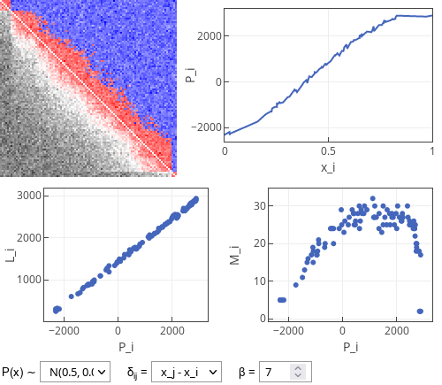
Fig. 1:Results of a simulation of the dynamic model showing the dependence of the newly introduced observables.

Interactive app

In the interactive app below you can see four plots. The top left plot is the "relationship" (or "popularity") matrix between the individual users. Its each row corresponds to user giving reaction and each column corresponds to user receiving reaction. In this plot blue color indicates at least one one-sided like given to another user (more intense blue indicates more likes given). Similarly red color indicates a match (users having positive balance of likes and dislikes with each other), while the more intense red corresponds to more likes. Dark gray colors indicate that a user has given more dislikes than likes to the receiving user (darker color indicates more negative balance). Note that the users in this plot are sorted from the least attractive (top rows) to the most attractive (bottom rows).

The top right plot shows the dependence between attractiveness and overall popularity of the user. As time goes the range observed popularity values increases. When plotting top left plot, we scale those values based on the current maximum and minimum value.

The bottom left plot shows the dependence between overall popularity of the user and total number of likes received by the user. Both of the observed variables change significantly in time.

The bottom right plot shows how the popularity of the user affects number of matches user gets. Most popular users are the ones most attractive, hence they get fewer matches.

References

• F. Olmeda. Towards a statistical physics of dating apps. arXiv:2107.14076 [physics.soc-ph].