Noise generated by a single charge carrier

Shot noise can be observed in variety of materials, devices and systems. Let us consider one of the simplest examples from physics: noise generated by trapping and detrapping of a single charge carrier.

Telegraph signal

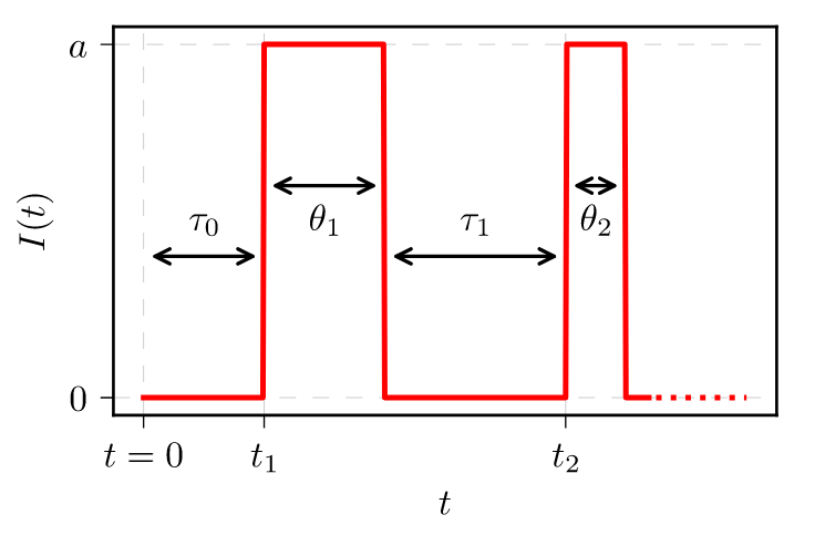
Let us postulate that if a charge carrier is free, then a flow of current is observed. Likewise, if the charge carrier is trapped, then the flow stops. Thus we are observing a signal with non-overlapping rectangular pulses (as shown in the figure below). Note that such signal is reminiscent of a telegraph signal.

Fig 1.Fragment of a signal with non-overlapping rectangular pulses.

The term trapping time is used for the time the charge carrier spends free (as it describes the time it takes for the charge carrier to be trapped). We use symbol \( \theta \) to denote it. The symbol \( \tau \) is used to denote the time it takes the charge carrier to escape. Effectively this means that charge carrier is detrapped, and thus the term detrapping time is used.

Poissonian random telegraph noise

As we have seen before simplest physical assumption would be that the escape probability is uniform in time (namely, that there are no ageing effects. This leads to a mathematical assumption that trapping and detrapping times follow exponential distribution with respective parameters \( \lambda_\theta \) (trapping rate) and \( \lambda_\tau \) (detrapping rate).

Derivation of the spectral density is a bit more involved than for the Poisson point process, but follows exactly the same trail of complex algebra. The general result (e.g., obtained in [1]) is

\begin{equation} S\left(f\right)=\frac{a^{2}\bar{\nu}}{\pi^{2}f^{2}}\mathrm{Re}\left[\frac{\left(1-\chi_{\theta}\left(f\right)\right)\left(1-\chi_{\tau}\left(f\right)\right)}{1-\chi_{\theta}\left(f\right)\chi_{\tau}\left(f\right)}\right], \end{equation}

with \( \chi_\theta(f) \) and \( \chi_\tau(f) \) standing for the characteristic functions of trapping and detrapping time distributions. As for the exponential distribution (with rate \( \lambda \)) we have

\begin{equation} \chi(f) = \frac{\lambda}{\lambda - 2 \pi \mathrm{i} f} , \end{equation}

the spectral density will have Lorentzian shape:

\begin{equation} S\left(f\right)=\frac{4a^{2}\bar{\nu}}{\left(\lambda_{\theta}+\lambda_{\tau}\right)^{2}+4\pi^{2}f^{2}}. \end{equation}

Namely, for low frequencies (lower than \( \left(\frac{\lambda_\theta + \lambda_\tau}{2 \pi}\right)^2 \)) the spectral density will be flat, while for higher frequencies \( S(f) \) will decay as \( 1/f^2 \). There will be a very narrow region of frequencies where the switch between the white noise and Brownian-like noise occurs.

Interactive app

Let us verify the analytical result by doing numerical simulation. The numerical results are shown as red curves (series in the top plot, and spectral density in the bottom plot) and theoretical curve is plotted in black (present only in the bottom plot). Note that as you change the rates the frequency at which the transition occurs changes, but the effect is symmetric (namely, for the spectral density plot it doesn't matter which rate you change).

Note: The app was recently updated with an additional parameter \( N_{success} \). It will be discussed in a forthcoming post (the link will be added after that post is published). When exploring the app in the context of this post simply keep the default \( N_{success} = 1 \).

References

• A. Kononovicius, B. Kaulakys. 1/f noise from the sequence of nonoverlapping rectangular pulses. Physical Review E 107: 034117 (2023). doi: 10.1103/PhysRevE.107.034117. arXiv:2210.11792 [cond-mat.stat-mech].