Accidental politicians

Over the last few posts I have been writing about variety of research conducted by a group based in University of Catania. I have covered some of their models illustrating various often counter-intuitive effects of randomness within social systems. This time let us talk about how a certain degree of randomness could benefit our political life [1].

Model

In accidental politicians model [1] the aim is to simulate effectiveness of legislatures under different scenarios. Each legislature is composed from \( N \) politicians (we use \( N = 141 \), because this is the number of politicians in Lithuanian parliament). Some of the politicians are independent, \( N_{ind} \), while the others are split between majority and minority parties or coalitions (the proportion is set by model parameter \( \rho_{maj} \).

Setting up legislature

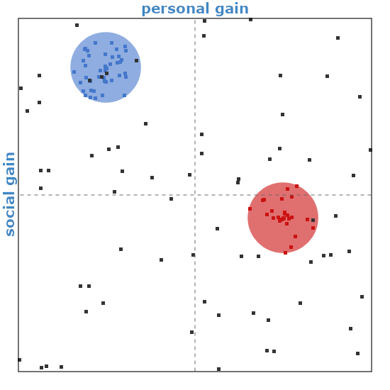
Each politician is characterized by their party affiliation (or lack of thereof), and by their position on personal-social gain graph. Position of independent politicians is set completely randomly (both coordinates are sampled uniformly from \( [-1, 1] \) value range, i.e., from \( \mathcal{U}(-1,1) \)), while affiliated politicians must be within the range of values tolerated by their party (i.e., at most \( r_{tol} \) from the party "ideal"). In the app below, parties are shown as big blue (majority) and red (minority) circles (the size of the circles indicates the range of tolerance, while the center coincides with the party "ideal"). Likewise affiliated politicians are shown as blue and green squares, which appear strictly within the circles. Independent politicians are shown as black squares, and they may be located anywhere on the personal-social gain graph.

Fig. 1:Freshly generated legislature. Small squares represent politicians, big circles - majority and minority parties. Horizontal axis is the personal gain axis. Vertical axis is the social gain axis.

Enacting laws

To simplify the presentation we have add additional parameter \( N_L \), which set the number of laws each legislature will vote on. After \( N_L \) laws have been voted on, a new election will occur and new politicians will be generated. In the app below we use \( N_L = 100 \), as this is large enough number to see what each particular legislature is about, and it is also small enough for quick simulation.

Law proposals are submitted by randomly selected politicians. Each proposal inherits social gain value of the proposer. Party affiliation of the proposer is also recorded. Members of the same party will always vote for a proposal submitted by their colleague. Members of the other party and independents will check the proposal a bit more thoroughly.

Member of the other party will vote for the proposal, if the social gain value of the proposal is greater than or equal to their party's "ideal" social gain, \( y \geq y_{id} \), and if they perceive that the personal gain is also greater than or equal to their party's "ideal", \( x_{id} \). Perception is implemented by randomizing proposal's personal gain coordinate, \( x^{\ast} \sim \mathcal{U}(-1, 1) \), for every politician. Thus the second condition would be \( x^{\ast} \geq x_{id} \). In other words, if social gain of the proposal is sufficiently high, a politician belonging to the other party will vote for the proposal with probability equal to \( \frac{x_{id} + 1}{2} \).

If the proposer was an independent, then all affiliated politicians would vote following this logic.

Independents ignore the party affiliation of the proposer. They always consider social gain and personal gain of the proposal using the logic outlined above. Though instead of using party "ideal" as a reference, they use their own coordinates.

The law is enacted if half or more of the politicians vote for it. If it is enacted, its social gain is added to the overall social welfare. Mathematically, we could track parliament history by storing voting outcomes as \( S_k \) (0 - failed vote, 1 - successful vote) and recording social gain values of the proposals as \( y_k \). Social welfare is then given by

\begin{equation} W_k = \sum_{i=0}^{k} S_i y_i . \end{equation}

For mathematical simplicity let us agree that \( W_{-1} = 0 \).

Example proposal

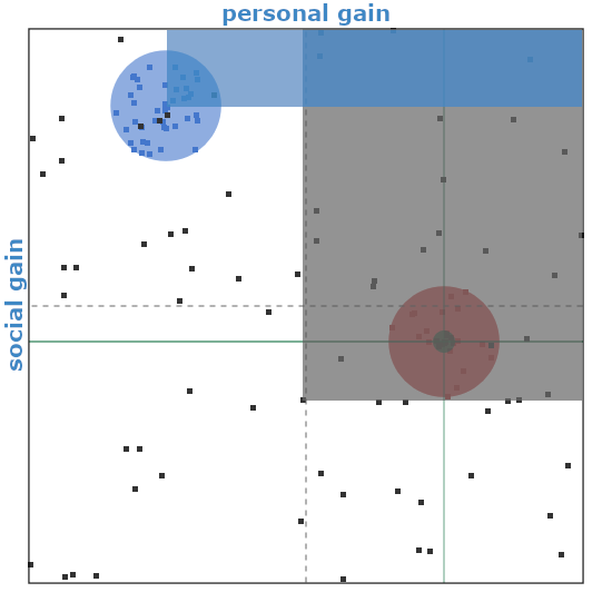
As an example let us consider the picture in the figure below. Proposer was randomly selected to be a member of the minority (red) party. Proposer is highlighted by a green circle. They are close to their party's "ideal", but the proposal inherits coordinates of the individual proposer.

Fig. 2:How a law proposal is being considered. Green circle corresponds to the coordinates of the proposer, while green lines help us estimate the coordiantes on the horizontal and vertical axes. Blue rectangle shows shared consideration window of the members of the minority party. Gray rectangle shows consideration window of an independent politician.

As the proposer is from the minority party, all the representatives of this paper will vote for the proposer.

Representatives of the majority (blue) party will not support this law, because social gain score of this proposal (which is in fact negative) is less than their "ideal" social gain, i.e., we have \( y < y_{id} \).

Independents will consider voting for the proposal only if the proposal's social gain score is greater than their own "ideal" social gain, i.e., \( y \geq y_{id} \). In this particular case, it is obvious that for most independents this condition does not hold, but it holds for the independent politician whom we have decided to highlight. Their consideration window is shown as gray rectangle. Notably, it is not necessary for the proposer to come from the consideration window, at this point it sufficient that social gain score of the proposal is greater than the independents expectation. Now, we would randomize personal gain (horizontal) coordinate of the proposal. If after this randomization the proposal remains in the consideration window, then the politician would vote to enact the proposal. Though as we can see in this particular case there is roughly \( 50\% \) chance of this happening.

In the simulation this proposal was not passed. Mostly because it was rejected by the majority's party's members, but also because of its low social gain score prevented independents to seriously consider it.

Calculating efficiency

So, after the law is enacted, its social gain is added to the social welfare. We could say that the most effective legislature is the one which increases social welfare the fastest. So it is natural to define efficiency as average social gain gained per proposal during the legislature. Mathematically efficiency of \( j \)-th legislature is given by

\begin{equation} E_j = \frac{W_{(j+1) N_L - 1} - W_{j N_L - 1}}{N_L} = \frac{1}{N_L} \sum_{i=0}^{N_L-1} S_{j N_L + i} y_{j N_L + i} . \end{equation}

In the above \( S_k \) is the success indicator of \( k \)-th proposal (this index spans across legislatures). Similarly, \( y_k \) is social gain value of the \( k \)-th proposal.

Results

I will not show lots of figures in this post, you can reproduce relevant points yourselves. Here instead, I'll just repeat the main conclusion of [1]. There is an optimal number of independent politicians,

\begin{equation} N^{\ast}_{ind} \approx \frac{4 N \rho_{maj} - 2 N - 4}{4 \rho_{maj} - 1} . \end{equation}

With this number of independent politicians the expected (or mean observed) efficiency of the legislature will be maximized. As far as I have tested, this result is well reproduced by the interactive app below.

With \( N = 141 \) and \( \rho_{maj} = 0.6 \) the optimal number of independents is between 37 and 38. As \( \rho_{maj} \) increases, then more independents are needed to reach optimal efficiency.

Interactive app

This app has quite a few graphs and plots. The descriptions below the app are helpful, so I would advise to look through them before proceeding to your own experimentation.

On the top-most row you will see average efficiency over all legislatures during the current simulation. Number of previously simulated legislatures is also provided for your interest.

In the top-left you can see the snapshot of the current legislature. If you decide to go slower, the last proposer would also be highlighted. Identically as in the figures above.

In the top-right you can see the efficiency-acceptance graph. The dots there show the average legislature efficiency conditioned on the observed acceptance for that legislature. The lines indicate how spread out the efficiency was with that acceptance.

The mid-row contains two frequency plots. They provide detailed information on how relatively often given efficiency and acceptance values were observed.

The bottom-row contains social welfare, \( W \), time series plot. It will show just the last \( N_L \) values. If you go at the top speed, you will see just the time series for the last legislature.

In the button-row there is an additional button, which allows the app user to switch between three distinct speeds (100 proposals per second, 400 proposals per second, 2000 proposals per second). The text on the button indicates the speed you could presently switch to.

References

• A. Pluchino, C. Garofalo, A. Rapisarda, S. Spagano, M. Caserta. Accidental Politicians: How Randomly Selected Legislators Can Improve Parliament Efficiency. Physica A 390: 3944-3954 (2011). doi: 10.1016/j.physa.2011.06.028. arXiv:1103.1224 [physics.soc-ph].