Long-range memory stochastic model of return

From the practical point of view price is the most interesting observable of the financial markets. Though modeling and analysis of price fluctuations are hindered by the fact that price itself is non-stationary process - mean price and market volatility constantly change. While price changes, at least at short time scales, behave as stationary process - mean price change is equal, or at least approximately equal, to zero. Thus it is convenient to introduce variable related to the relative price changes, which is known as return

\begin{equation} r (t, \Delta t) = \ln \left[ \frac{p(t)}{p(t-\Delta t)}\right] . \end{equation}

If the change of price, \( p(t)-p(t-\Delta t) \), is small, then the above definition of return is analogous to relative price change, \( \frac{p(t)-p(t-\Delta t)}{p(t-\Delta t)} \).

There are few very common and general statistical properties of return. Those statistical properties, also called stylized facts, were established while analyzing return time series of different stocks from different markets all over the world.

One of those facts is fat tails, leptocurtic, of return distribution. Fatter than Gaussian empirical return distribution tails are most usually fitted using power law functions (powers fluctuate between 3 and 4). In this text we use q-Gaussians, which are known to fit return distributions in whole range of return values [1] - not only the tail region as simple power law functions do.

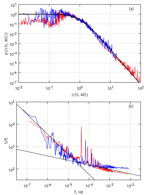
It is also known that autocorrelation of absolute return time series decays very slowly - as power law. While the spectral density of absolute return time series is known to be double power law - smaller frequencies are fitted with power 0.9, while larger can be fitted with power 0.2. In the figure below, Fig. 1, we have show aforementioned statistical properties of one minute absolute returns observed in New York (red line) and Vilnius (blue line) Stock Exchanges.

Fig. 1:Statistical properties of absolute one minute, Δt=60s, returns - probability density function of non-zero values (a) and power spectral density (b) - from two different financial markets. Red curves represent New York Stock Exchange, while blue correspond to statistical properties of return in Vilnius Stock Exchange. Black curves approximate empirical data - (a) q-Gaussian (q=1.55), (b) power law functions (powers 0.9 and 0.2).

Note that in Fig. 1 statistical properties of different financial markets slightly differ. This happens mainly due to the fact that time interval of return, \( \Delta t \), is significantly larger than mean inter-trade time in New York Stock Exchange (approximately 3 seconds), but in case of Vilnius Stock Exchange \( \Delta t \) is smaller than mean inter-trade time (approximately 362 seconds). Thus most of one minute time intervals in New York Stock Exchange contain deals and price changes (75% of time intervals have non-zero return), while majority of one minute time intervals in Vilnius Stock Exchange are empty (92% of time intervals have zero return). That is why spectral densities of two stock exchanges slightly disagree, and the reason why we must compare probability density functions of non-zero values.

In the next sections of this text we will replicate derivation of long range memory stochastic model of return. Later in this work we will also present interactive Java applet. The model and related works are discussed in [2] reference.

Langevin equation with q-Gaussian stationary distribution

From the stochastic analysis (see for example [3]) it is known that, if in general case Langevin equation can be written as

\begin{equation} \mathrm{d} r = f(r) \mathrm{d} t + g(r) \mathrm {d} W , \end{equation}

then stationary distribution of this equation is

\begin{equation} p (r) = \frac{1}{g^2(r)} \exp \left[ 2 \int\frac{f(r)}{g^2(r)} \mathrm{d} r \right] . \end{equation}

The above relation can be re-expressed in differential terms with respect to one of the functions from Langevin equation, \( f(r) \) or \( g(r) \),

\begin{equation} f(r) = \frac{1}{2} g^2(r) \frac{\partial_r p(r)}{p(r)} +g(r) \partial_r g(r) . \end{equation}

This differential relation is needed as we know that stationary distribution must be q-Gaussian (more transparent form is obtained in [2]). \( g(r) \) we can choose freely, thus in agreement with previous work \( g(r) = \sigma (r_0^2 +r^2)^{\frac{\eta}{2}} \) is chosen. At this point we can already write Langevin equation for return. Though by making some substitutions, \( x=\frac{r}{r_0} \), \( t_s = \sigma^2 r_0^{2(\eta - 1)} t \), we can obtain dimensionless stochastic differential equation

\begin{equation} \mathrm{d} x = \left ( \eta - \frac{\lambda}{2} \right)\left( 1+x^2 \right)^{\eta-1} x \mathrm{d} t + \left( 1+x^2\right)^{\frac{\eta}{2}} \mathrm{d} W . \end{equation}

The equation above describes dynamics of momentary return, while we are interested in compounded return. Thus the solutions of the above equation must be integrated in chosen time intervals, \( \tau \),

\begin{equation} X(t) = \frac{1}{\tau} \left | \int\limits_{t}^{t+\tau}x(s) \mathrm{d} s \right | . \end{equation}

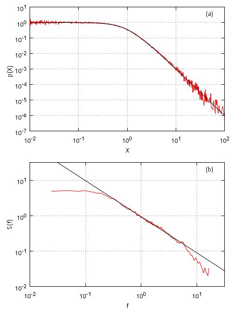
The above stochastic differential equation reproduces time series with q-Gaussian stationary distribution (power fitting the tail is \( \lambda \)) and power law spectral density - in one region approximated by power law function with power \( \beta = 1 - \frac{3 -\lambda}{2 (\eta-1)} \) (see [4]). By manipulating with model parameter \( \lambda \) and \( \eta \) values one can obtain almost any spectra with \( \beta \in [0.5,2] \). As an example we provide 1/f spectral density (see Fig. 2b).

Fig. 2:1/f noise obtained from the above SDE. Red curves correspond to model statical properties (probability density function (a), spectral density (b)), while black curves fit modelic statistical properties (q-Gaussian, q=1.66, (a), power law function, β=1, (b)). Used model parameters: λ=3, η=1.5, τ=0.02. Model statistical properties averaged over 100 realizations containing 4096 points.

Langevin equation with double power law spectral density

Though results presented in Fig. 2 are already astonishing, but as we saw in Fig. 1b power spectral density of absolute return is fractured (containing two different power law regions). To reproduce the fracture one must to divide space of \( x \) diffusion into two different multiplicativity regions. Improved stochastic differential equation, with two powers of multiplicativy, can be written as

\begin{equation} \mathrm{d} x = \left ( \eta - \frac{\lambda}{2} \right)\frac{\left( 1+x^2 \right)^{\eta-1}}{\left( 1 + \epsilon\sqrt{1+x^2} \right)^2} x \mathrm{d} t + \frac{\left( 1+x^2\right)^{\frac{\eta}{2}}}{1 + \epsilon \sqrt{1+x^2}} \mathrm{d}W , \end{equation}

here \( \epsilon \) parameter controls division of \( x \) diffusion space. One can introduce into the above equation new terms, which would restrict diffusion of \( x \). If those terms are not introduced one would need to limit numerical solutions using min and max functions available in most programing languages. We propose to introduce \( - \left( \frac{x}{x_{max}} \right)^2 \) (this is default variation used in the most recent articles) or \( - (x \epsilon)^2 \) (this is non-default variation, which was used in our first article concerned with return modeling).

Introduction of q-Gaussian noise

Yet still solutions of the above equation appear to be smoother than empirical time series [2] - difference between power laws approximating model spectra are minor, while in the time domain model return fluctuates as slow continuous function. Similar behavior is demonstrated by the moving average of actual return. Thus this encourages us to proposed to decompose return into two very different processes - slow long-range memory process (described by Langevin equation) and fast large fluctuation process (noise).

Empirical analysis [2] shows that fast fluctuations is also q-Gaussian, \( r = \zeta \left( r_0 ,\lambda_2 \right) \). Power, \( \lambda_2 \) of the distribution tail appears to be constant and equal to 5. While \( r_0 \), responsible for variance in time series, appears to be linearly related to the moving average of return, \( MA(r(t)) \),

\begin{equation} r_0(MA(r(t))) = 1 + 2 \left | MA(r(t)) \right | . \end{equation}

As \( MA(r(t)) \) seems to behave similarly to \( X \) we can rewrite above relation as

\begin{equation} r_0 (t) = 1 + \frac{\bar {r_0}}{\tau_s} \left |\int\limits_{t_s}^{t_s + \tau_s} x(s) \mathrm{d} s \right | , \end{equation}

here \( \bar {r_0} \) is model parameter bearing the meaning of mean return per unit time interval.

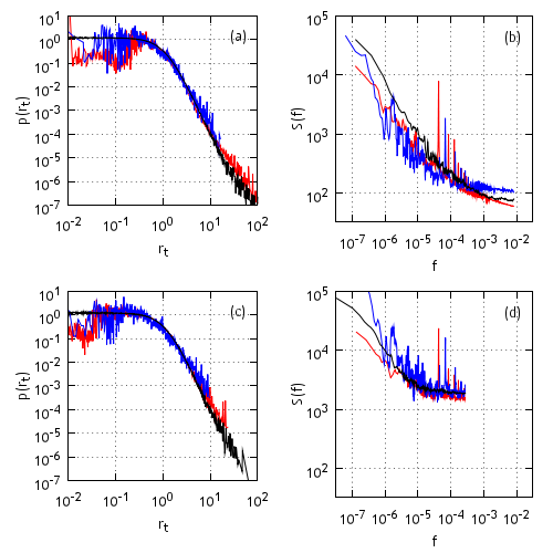
Thus now we first solve stochastic differential equation, then we integrate its solutions in some intervals and then modulate those solutions with q-Gaussian noise. Results obtained in this way is in great agreement with empirical data (see Fig. 3).

Fig. 3:Comparison of return model (black curve) and empirical (New York Stock Exchange - red curve, Vilnius - blue) statistical properties, non-zero value probability density function ((a) ir (c)) and power spectral density ((b) ir (d)), in different time scales (1 min - (a) and (b), 30 min - (c) and (d)). Model parameters: \( \tau_s =2 \cdot 10^{-4} \) (1 min) and \( τ_s=6 \cdot 10^{-3} \) (30 min), \( λ_2 = 5 \), \( {\bar r}_0=0.4 \), \( \lambda=3.6 \), \( \varepsilon =0.017 \), \( \eta =2.5 \), \( x_{max}=1000 \).

Applet

HTML5 applet below solves differential equations above using Euler-Maruyama method [5]. We also use variable time step. In such case stochastic differential equations becomes a set of difference equations for time and return. In case of the last stochastic differential above

\begin{equation} x_{i+1} = x_{i} + \kappa^2 \left [ \eta -\frac{\lambda}{2} - \left( \frac{x_i}{x_{max}} \right)^2\right] x_i + \kappa \sqrt{1+x_i^2} \xi_i , \end{equation}

\begin{equation} t_{i+1} = t_{i} + \kappa^2 \frac{\left( 1 + \epsilon\sqrt{1+x_i^2} \right)^2}{\left( 1+x_i^2 \right)^{\eta-1}}, \end{equation}

here \( \xi_i \) is Gaussian noise (zero mean, unit variance) and \( \kappa \) is numerical precision parameter.

You can also download a full java program with GUI in Lithuanian or English language (the code for this GUI program is also available from GitHub). Note that only GUI was localized - meaning that CLI is English in both cases.

References

• Cf. M. Gell-Mann, C. Tsallis. Nonextensive Entropy - Interdisciplinary Applications. Oxford University Press, New York, 2004.
• V. Gontis, J. Ruseckas, A. Kononovicius. A Non-linear Stochastic Model of Return in Financial Markets. In: Stochastic Control, ed. C. Myers. InTech, 2010. doi: 10.5772/9748.
• C. W. Gardiner. Handbook of stochastic methods. Springer, Berlin, 2009.
• B. Kaulakys, M. Alaburda. Modeling scaled processes and \\\( 1/f^\beta \\\) noise using non-linear stochastic differential equations. Journal of Statistical Mechanics, 2009: P02051. arXiv: 1003.1155 [nlin.AO].
• P. E. Kloeden, E. Platen. Numerical Solution of Stochastic Differential Equations. Springer, Berlin, 1999.